Auditory cortex working model#

Localization and parcellation of the auditory cortex#

As mentioned before, we are interested in the functional organization of the human auditory cortex and thus want to restrict our analyses to the corresponding region. The question of choosing the “right” region(s) is not an easy one and is actively discussed throughout neuroimaging. The auditory cortex is no exception to that, to the contrary: its localization and parcellation are even less standardized and agreed on than other primary sensory regions (e.g. visual and motor cortex), which is part of the reason we conducted this meta-analytic approach. So, in order to get started we need at least a rough working model of “where” the human auditory cortex is, to then investigate its functional organization. Given that structural markers were found to be more consistent regarding the localization of the auditory cortex and we did not want to incorporate task/analyses based biases, we decided to base our general outline on a structural brain atlas from which we could extract regions that are frequently reported with regard to auditory brain function. Additionally targeting a trade-off between parsimonious and fine-grained solutions, we utilized the Harvard-Oxford-Atlas within our project. It allowed us to extract and subsequently combine regions to create an auditory cortex mask that covered the upper 2/3 of the temporal lobe, including the Superior Temporal Plane (STP) and Superior Temporal Gyrus (STG). In more detail, it entailed the following ROIs:

Heschl gyrus (HG)
Planum Polare (PP)
Planum Temporale (PT)
anterior Superior Temporal Gyrus (aSTG)
posterior Superior Temporal Gyrus (pSTG)

This section of the walkthrough will provide detailed steps and code on how these regions were extracted from the Harvard-Oxford-Atlas and subsequently combined to form the auditory cortex mask. We’ll use nipype & nilearn functionality to do so. This mask was the basis for all analyses as we determined the meta-analytic functional profile for all voxels within it from which we then derived different cluster solutions which were used for co-activation analyses and functional profile decoding, as well as an affinity matrix which was used for the computation of meta-analytic gradients.

However, at first we need to import necessary modules and functions.

Import necessary modules and functions#

import os
from os.path import join as opj
import nibabel as nb
from nilearn import datasets
from nilearn.image import math_img
from nilearn.plotting import plot_anat
from nipype.pipeline import Node
from nipype.algorithms.misc import PickAtlas
import matplotlib.pyplot as plt
from matplotlib.lines import Line2D
from matplotlib import colors
import seaborn as sns

%matplotlib inline

Obtain the atlas and extract ROIs#

Initially, we’ll download the Harvard-Oxford atlas using nilearn:

dataset_harvard_oxford = datasets.fetch_atlas_harvard_oxford('cort-maxprob-thr25-2mm')
atlas_filename_harvard_oxford = dataset_harvard_oxford.maps

To extract our ROIs, we need to know their name, label and/or number in the given parcellation. Let’s gather this information:

for labels_harvard_oxford in enumerate(dataset_harvard_oxford.labels):
    print(labels_harvard_oxford)

(0, 'Background')
(1, 'Frontal Pole')
(2, 'Insular Cortex')
(3, 'Superior Frontal Gyrus')
(4, 'Middle Frontal Gyrus')
(5, 'Inferior Frontal Gyrus, pars triangularis')
(6, 'Inferior Frontal Gyrus, pars opercularis')
(7, 'Precentral Gyrus')
(8, 'Temporal Pole')
(9, 'Superior Temporal Gyrus, anterior division')
(10, 'Superior Temporal Gyrus, posterior division')
(11, 'Middle Temporal Gyrus, anterior division')
(12, 'Middle Temporal Gyrus, posterior division')
(13, 'Middle Temporal Gyrus, temporooccipital part')
(14, 'Inferior Temporal Gyrus, anterior division')
(15, 'Inferior Temporal Gyrus, posterior division')
(16, 'Inferior Temporal Gyrus, temporooccipital part')
(17, 'Postcentral Gyrus')
(18, 'Superior Parietal Lobule')
(19, 'Supramarginal Gyrus, anterior division')
(20, 'Supramarginal Gyrus, posterior division')
(21, 'Angular Gyrus')
(22, 'Lateral Occipital Cortex, superior division')
(23, 'Lateral Occipital Cortex, inferior division')
(24, 'Intracalcarine Cortex')
(25, 'Frontal Medial Cortex')
(26, 'Juxtapositional Lobule Cortex (formerly Supplementary Motor Cortex)')
(27, 'Subcallosal Cortex')
(28, 'Paracingulate Gyrus')
(29, 'Cingulate Gyrus, anterior division')
(30, 'Cingulate Gyrus, posterior division')
(31, 'Precuneous Cortex')
(32, 'Cuneal Cortex')
(33, 'Frontal Orbital Cortex')
(34, 'Parahippocampal Gyrus, anterior division')
(35, 'Parahippocampal Gyrus, posterior division')
(36, 'Lingual Gyrus')
(37, 'Temporal Fusiform Cortex, anterior division')
(38, 'Temporal Fusiform Cortex, posterior division')
(39, 'Temporal Occipital Fusiform Cortex')
(40, 'Occipital Fusiform Gyrus')
(41, 'Frontal Operculum Cortex')
(42, 'Central Opercular Cortex')
(43, 'Parietal Operculum Cortex')
(44, 'Planum Polare')
(45, "Heschl's Gyrus (includes H1 and H2)")
(46, 'Planum Temporale')
(47, 'Supracalcarine Cortex')
(48, 'Occipital Pole')

As we can see, the regions we are interest in have the following labels:

HG - 45
PP - 44
PT - 46
aSTG - 9
pSTG - 10

While other atlases distinguish hemispheres on the label level, the one we’re using does not. Therefore, we need to specify the hemisphere in the function that extracts the ROIs from the atlas. For this, we’ll employ nipype’s PickAtlas function. As we want to extract multiple ROIs from the same atlas, we’ll set up a general ROI extraction node, defining only the input atlas and create clone nodes for each ROI respectively. Here’s the setup for the general ROI extraction node:

extract_ROIs_harvard_oxford = Node(PickAtlas(), name='extract_ROIs_harvard_oxford')
extract_ROIs_harvard_oxford.inputs.atlas = atlas_filename_harvard_oxford

If we, for example, want to extract the left hemisphere HG, the ROI specific cloned node would look as follows:

## setup ROI specific node - HG left
extract_ROIs_harvard_oxford_HG_left = extract_ROIs_harvard_oxford.clone(name='extract_ROIs_harvard_oxford_HG_left')
extract_ROIs_harvard_oxford_HG_left.inputs.hemi = 'left'
extract_ROIs_harvard_oxford_HG_left.inputs.labels = 45
extract_ROIs_harvard_oxford_HG_left.inputs.output_file = 'prerequisites/ac_rois/tpl-MNI152NLin6Sym_res_02_desc-HGleft_mask.nii.gz'

## run node
extract_ROIs_harvard_oxford_HG_left.run()

## check if ROIs was extracted and saved
os.listdir('prerequisites/ac_rois/')

['tpl-MNI152NLin6Sym_res_02_desc-HGleft_mask.nii.gz']

Great, that seems to work. Now let’s extract the remaining ROIs. As we’re lazy, we’re going to do this within a small for-loop instead of running it one by one manually:

roi_name_tpl = 'prerequisites/ac_rois/tpl-MNI152NLin6Sym_res_02_desc-'

for hemi in ['left', 'right']:
    for label, name in zip([45,44,46,9,10], ['HG', 'PP', 'PT', 'aSTG', 'pSTG']):
        print('extracting ROI %s with label %s from %s hemisphere' %(name, label, hemi))
       
        ##set up node
        extract_ROIs_harvard_oxford_tmp = extract_ROIs_harvard_oxford.clone(name='extract_ROIs_harvard_oxford_tmp')
        extract_ROIs_harvard_oxford_tmp.inputs.hemi = hemi
        extract_ROIs_harvard_oxford_tmp.inputs.labels = label
        extract_ROIs_harvard_oxford_tmp.inputs.output_file = '%s%s%s_mask.nii.gz' %(roi_name_tpl, name, hemi)

        ## run node
        extract_ROIs_harvard_oxford_tmp.run()
        
        del extract_ROIs_harvard_oxford_tmp
        
## check if ROIs were extracted and saved
os.listdir('prerequisites/ac_rois/')

['tpl-MNI152NLin6Sym_res_02_desc-aSTGleft_mask.nii.gz',
 'tpl-MNI152NLin6Sym_res_02_desc-aSTGright_mask.nii.gz',
 'tpl-MNI152NLin6Sym_res_02_desc-pSTGright_mask.nii.gz',
 'tpl-MNI152NLin6Sym_res_02_desc-HGright_mask.nii.gz',
 'tpl-MNI152NLin6Sym_res_02_desc-PPleft_mask.nii.gz',
 'tpl-MNI152NLin6Sym_res_02_desc-HGleft_mask.nii.gz',
 'tpl-MNI152NLin6Sym_res_02_desc-pSTGleft_mask.nii.gz',
 'tpl-MNI152NLin6Sym_res_02_desc-PTright_mask.nii.gz',
 'tpl-MNI152NLin6Sym_res_02_desc-PTleft_mask.nii.gz',
 'tpl-MNI152NLin6Sym_res_02_desc-PPright_mask.nii.gz']

Having extracted all the ROIs we wanted to include, we can now also combine into a new file which will be the mask we’re going to use in the planned searchlight analyses. To do so, we’re going to use nilearn again, more precisely it’s math_img functionality.

Merge ROIs to create an auditory cortex mask#

To save some space, we’ll define the path to the ROIs:

ROI_path = 'prerequisites/ac_rois/'

Next, we load all ROIs:

HG_left = nb.load(opj(ROI_path, 'tpl-MNI152NLin6Sym_res_02_desc-HGleft_mask.nii.gz'))
HG_right = nb.load(opj(ROI_path, 'tpl-MNI152NLin6Sym_res_02_desc-HGright_mask.nii.gz'))
PP_left = nb.load(opj(ROI_path, 'tpl-MNI152NLin6Sym_res_02_desc-PPleft_mask.nii.gz'))
PP_right = nb.load(opj(ROI_path, 'tpl-MNI152NLin6Sym_res_02_desc-PPright_mask.nii.gz'))
PT_left = nb.load(opj(ROI_path, 'tpl-MNI152NLin6Sym_res_02_desc-PTleft_mask.nii.gz'))
PT_right = nb.load(opj(ROI_path, 'tpl-MNI152NLin6Sym_res_02_desc-PTright_mask.nii.gz'))
aSTG_left = nb.load(opj(ROI_path, 'tpl-MNI152NLin6Sym_res_02_desc-aSTGleft_mask.nii.gz'))
aSTG_right = nb.load(opj(ROI_path, 'tpl-MNI152NLin6Sym_res_02_desc-aSTGright_mask.nii.gz'))
pSTG_left = nb.load(opj(ROI_path, 'tpl-MNI152NLin6Sym_res_02_desc-pSTGleft_mask.nii.gz'))
pSTG_right = nb.load(opj(ROI_path, 'tpl-MNI152NLin6Sym_res_02_desc-pSTGright_mask.nii.gz'))

Now we can combine them into one mask:

ac_mask = math_img("HG_left+HG_right+PP_left+PP_right+PT_left+PT_right+aSTG_left+aSTG_right+pSTG_left+pSTG_right",
                           HG_left=HG_left, PP_left=PP_left, PT_left=PT_left, aSTG_left=aSTG_left, pSTG_left=pSTG_left,
                           HG_right=HG_right, PP_right=PP_right, PT_right=PT_right, aSTG_right=aSTG_right, pSTG_right=pSTG_right,)

ac_mask.to_filename(opj(ROI_path, 'tpl-MNI152NLin6Sym_res_02_desc-AC_mask.nii.gz'))

As we know that there will be some hemisphere specific analyses along our way, we’ll also create an auditory cortex mask for a given hemisphere. First, the left hemisphere:

ac_mask_left = math_img("HG_left+PP_left+PT_left+aSTG_left+pSTG_left",
                         HG_left=HG_left, PP_left=PP_left, PT_left=PT_left, aSTG_left=aSTG_left, pSTG_left=pSTG_left)

ac_mask_left.to_filename(opj(ROI_path, 'tpl-MNI152NLin6Sym_res_02_desc-ACleft_mask.nii.gz'))

And for the right hemisphere:

ac_mask_right = math_img("HG_right+PP_right+PT_right+aSTG_right+pSTG_right",
                          HG_right=HG_right, PP_right=PP_right, PT_right=PT_right, aSTG_right=aSTG_right, pSTG_right=pSTG_right,)

ac_mask_right.to_filename(opj(ROI_path, 'tpl-MNI152NLin6Sym_res_02_desc-ACright_mask.nii.gz'))

Given there is always some spatial uncertainty and mismatch concerning alignment and transformations, we will dilate the created masks by one voxel using FreeSurfer’s mri_binarize:

%%bash
mri_binarize --i prerequisites/ac_rois/tpl-MNI152NLin6Sym_res_02_desc-AC_mask.nii.gz --min 0.1 --o prerequisites/ac_rois/tpl-MNI152NLin6Sym_res_02_desc-ACdilated_mask.nii.gz --dilate 1
mri_binarize --i prerequisites/ac_rois/tpl-MNI152NLin6Sym_res_02_desc-ACleft_mask.nii.gz --min 0.1 --o prerequisites/ac_rois/tpl-MNI152NLin6Sym_res_02_desc-ACleftdilated_mask.nii.gz --dilate 1
mri_binarize --i prerequisites/ac_rois/tpl-MNI152NLin6Sym_res_02_desc-ACright_mask.nii.gz --min 0.1 --o prerequisites/ac_rois/tpl-MNI152NLin6Sym_res_02_desc-ACrightdilated_mask.nii.gz --dilate 1

Before we brashly assume that everything worked out, it would be a good idea to visually check our auditory cortex mask to make sure nothing is off. Once more, we’re lucky that nilearn exists, as it also comes with a lot of plotting functionalities.

Evaluating auditory cortex mask:#

In order to get a nice overview, we’ll plot the created auditory cortex mask on a template brain:

#suppress contour related warnings
import warnings
warnings.filterwarnings("ignore")

ac_mask = nb.load(opj(ROI_path, 'tpl-MNI152NLin6Sym_res_02_desc-ACdilated_mask.nii.gz'))

sns.set_style('white')
plt.rcParams["font.family"] = "Arial"   

fig=plt.figure(num=None, figsize=(12, 6))
check_mask = plot_anat(cut_coords=[-55, -34, 7], figure=fig, draw_cross=False)
check_mask.add_contours(ac_mask, 
                        levels=[0], colors='black')

plt.text(-215, 90, 'Auditory cortex mask',
         fontsize=22)

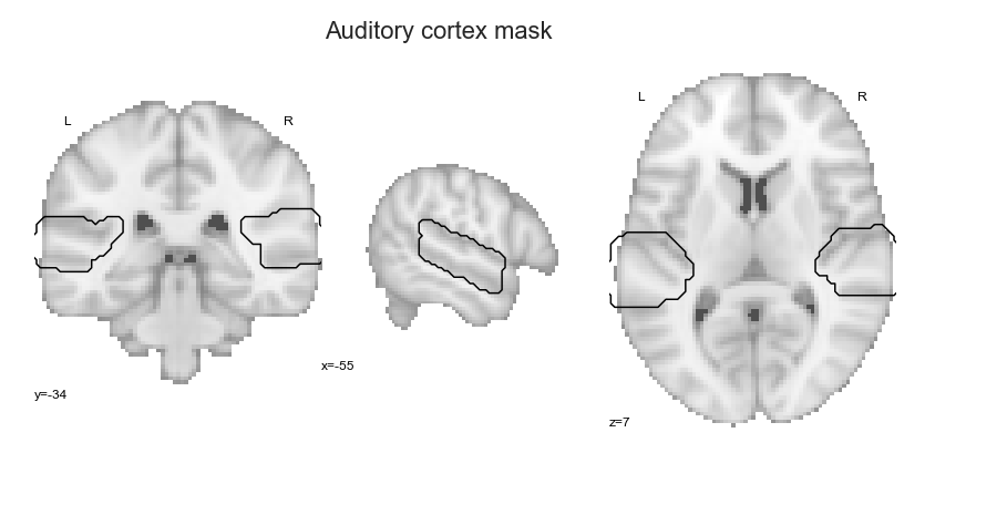
That looks about right! Now, we can start with the planned analyses, beginning with the clustering solutions.

Access the ROIs and masks#

Instead of rerunning the steps above and/or if you just want the ROIs and the masks, you can access these files in the form we used them in this section of the project’s OSF project.

Large scale meta-analyses of the Auditory Cortex - A Walkthrough

Auditory cortex working model

Contents