Co-activation analysis

Within this section the co-activation analyses, are shown, explained and set up in a way that they can be rerun and reproduced. In short, we employed the Neurosynth database again to compute and meta-analytic co-activation patterns for each cluster in our 5-cluster solution we obtained in the previous step. In a multistep procedure we investigated which voxels and regions are likely to co-activate with our clusters across studies in the Neurosynth database and via contrasting co-activation patterns evaluated if the clusters are part of functionally separable networks. The analysis was divided into the following sections:

Prerequisites

• Neurosynth database

• Cluster solution

• Auditory cortex mask

Co-activation analyses

• Per cluster

• Per cluster against entire AC

• Grouped clusters

• Per cluster between hemispheres

We provide more detailed information and explanations in the respective sections. As mentioned before, you can rerun the analyses either by downloading this page as a Jupyter Notebook (via the download button at the top) or interactively via a cloud instance through the amazing mybinder project (the little rocket at the top). We recommend the later to spare installation and conda environment related problems. We provide all co-activation maps (in volume and surface format) via the project’s OSF page and included all code and explanations depicting how this steps were run below. If folks want to just explore the co-activation maps, the respective code for downloading them is included in the respective sections.

First let’s import some basic necessities:

%matplotlib inline

from os.path import join as opj 
from copy import deepcopy
import numpy as np
from neurosynth.base.dataset import Dataset
from neurosynth.analysis.meta import MetaAnalysis

from neurosynth import mask
import nibabel as nb
from nilearn.image import math_img
from nilearn.input_data import NiftiMasker

import matplotlib.pyplot as plt
from matplotlib.colors import ListedColormap
from matplotlib.patches import Patch
from matplotlib.lines import Line2D

import seaborn as sns
from nilearn.plotting import plot_anat, plot_roi, plot_img, plot_stat_map, view_img, view_img_on_surf 

Prerequisites

Before we can start with the actual analyses, we need to define some prerequisites we are going to utilize throughout this section. For example, paths to the neurosynth dataset and the cluster solutions.

neurosynth_path = 'prerequisites/neurosynth'
cluster_path = 'parcellations'
ac_roi_path = 'prerequisites/ac_rois'
results_path = 'results/coactivation'

We are also going to set our default colormap that we will use throughout the analyses:

cmap_co = sns.cubehelix_palette(5, start=-.2, rot=.6, reverse=True, as_cmap=True)
cmap_co_sns = sns.cubehelix_palette(5, start=-.2, rot=.6, reverse=True)
cmap_co_list = ListedColormap(sns.cubehelix_palette(5, start=-.2, rot=.6, reverse=True))

Neurosynth dataset

With that set up, we can define and load everything we need, beginning with the neurosynth dataset we created in the previous step:

neurosynth_dataset = Dataset.load(opj(neurosynth_path,'neurosynth_dataset.pkl'))

We are going to make sure the dataset looks like in the clustering analyses:

neurosynth_dataset.activations.head(n=10)

	id	doi	x	y	z	space	peak_id	table_id	table_num	title	authors	year	journal	i	j	k
0	9065511	NaN	38.0	-48.0	49.0	MNI	548691	28698	1.	Environmental knowledge is subserved by separa...	Aguirre GK, D'Esposito M	1997	The Journal of neuroscience : the official jou...	60	39	26
1	9065511	NaN	-4.0	-70.0	50.0	MNI	548692	28698	1.	Environmental knowledge is subserved by separa...	Aguirre GK, D'Esposito M	1997	The Journal of neuroscience : the official jou...	61	28	47
2	9065511	NaN	-34.0	-52.0	60.0	MNI	548693	28698	1.	Environmental knowledge is subserved by separa...	Aguirre GK, D'Esposito M	1997	The Journal of neuroscience : the official jou...	66	37	62
3	9065511	NaN	-23.0	15.0	67.0	MNI	548694	28698	1.	Environmental knowledge is subserved by separa...	Aguirre GK, D'Esposito M	1997	The Journal of neuroscience : the official jou...	70	70	56
4	9065511	NaN	-23.0	-20.0	68.0	MNI	548695	28698	1.	Environmental knowledge is subserved by separa...	Aguirre GK, D'Esposito M	1997	The Journal of neuroscience : the official jou...	70	53	56
5	9065511	NaN	42.0	-47.0	-19.0	MNI	548696	28698	1.	Environmental knowledge is subserved by separa...	Aguirre GK, D'Esposito M	1997	The Journal of neuroscience : the official jou...	26	40	24
6	9065511	NaN	25.0	-35.0	-8.0	MNI	548697	28698	1.	Environmental knowledge is subserved by separa...	Aguirre GK, D'Esposito M	1997	The Journal of neuroscience : the official jou...	32	46	32
7	9065511	NaN	-25.0	-45.0	-2.0	MNI	548698	28698	1.	Environmental knowledge is subserved by separa...	Aguirre GK, D'Esposito M	1997	The Journal of neuroscience : the official jou...	35	40	58
8	9065511	NaN	52.0	-62.0	14.0	MNI	548699	28698	1.	Environmental knowledge is subserved by separa...	Aguirre GK, D'Esposito M	1997	The Journal of neuroscience : the official jou...	43	32	19
9	9065511	NaN	21.0	-81.0	28.0	MNI	548700	28698	1.	Environmental knowledge is subserved by separa...	Aguirre GK, D'Esposito M	1997	The Journal of neuroscience : the official jou...	50	22	34

Check, that looks about right.

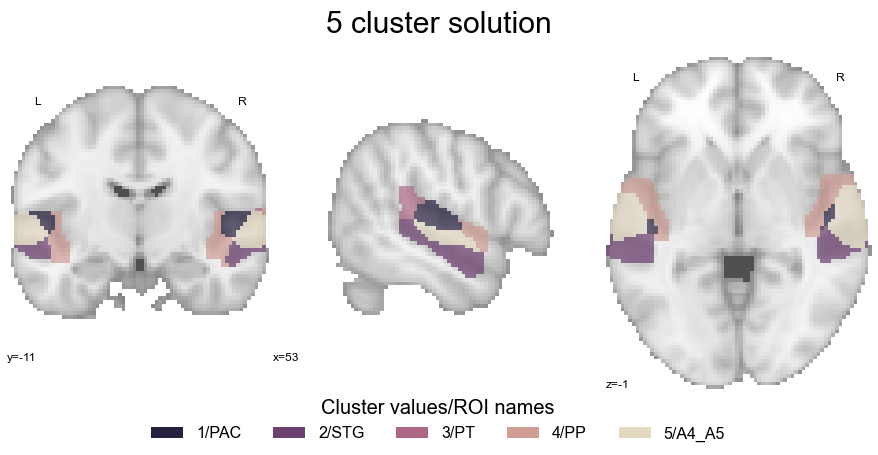
Cluster solution

We also need to define and load our chosen cluster solution, i.e. the 5 cluster solution.

cluster_solution= opj(cluster_path, '/opt/miniconda/envs/neurosynth-ac/lib/python3.6/site-packages/neurosynth/resources/tpl-MNI152NLin6Sym_atlas-nsac_desc-5.nii.gz')

Not that it was that long ago, but it might be a good idea to plot the cluster solution again here for consistency and easy access reasons:

plt.rcParams["font.family"] = "Arial"   

fig= plt.figure(figsize=(12, 6))

plot_roi(cluster_solution, cmap=cmap_co_list, draw_cross=False, figure=fig)

legend_elements = [Patch(facecolor=cmap_co_list(0), label='1/PAC'),
                   Patch(facecolor=cmap_co_list(1), label='2/STG'),
                   Patch(facecolor=cmap_co_list(2), label='3/PT'),
                   Patch(facecolor=cmap_co_list(3), label='4/PP'),
                   Patch(facecolor=cmap_co_list(4), label='5/A4_A5')]

plt.legend(handles=legend_elements, loc='lower center', bbox_to_anchor=(-0.63, -0.2), 
           frameon=False, ncol=5, title='Cluster values/ROI names', prop={'size': 16}, title_fontsize=20)

plt.text(-220,85, '5 cluster solution', fontsize=30)

Ok, great. Given that we also want to explore this cluster solution a bit more and the static volume view is a bit restrictive, we will also generate an interactive plot that allows us to scroll through the different views:

view_img(cluster_solution, cmap=cmap_co, symmetric_cmap=False, black_bg=False, colorbar=False)

Much more informative! We now have all prerequisites we need for the co-activation analyses set and ready to go. Thus, let’s do this!

Co-activation analyses

Having obtained the different meta-analyses based cluster solutions and decided on the "best solution given the data", the aim is to understand the clusters in more detail. This especially refers to if the clusters are functionally separable, that is if they reflect regions of the AC that entail distinct functionality that in turn can shed light on the organization of the AC. One possibility to do that and also utilize the rich information present in the neurosynth dataset again to provide a holistic overview based on large-scale data, is to compute so-called co-activation patterns. As hinted at in the introduction, meta-analytic co-activation analyses describe the probability of voxels and thus regions being co-activated with a given seed region (here the clusters in our solution) based on the studies included in the neurosynth dataset. In other words: for all voxels, what is the likelihood of being "active" given that e.g. cluster 1 was "active"? Here, this was extended via meta-analytic contrasts within which studies that activated one (set of) cluster(s) were contrasted against those that activated the opposing (set of) cluster(s). The resulting co-activation maps therefore indicated voxels and regions that were more frequently reported as activated when e.g. cluster 1 was active as compared to cluster 2, and vice versa. Luckily, we can once more build upon the neurosynth functionality and specifically the fantastic work of Alejandro de la Vega, who wrote a function that performs these meta-analytic contrasts and because he is amazing, shared it.

def mask_level(img, level):
    img = deepcopy(img)
    data = img.get_data()
    data[:] = np.round(data)
    data[data != level] = 0 
    data[data == level] = 1
    
    return img

def coactivation_contrast(dataset, infile, regions=None, target_thresh=0.01, 
                          other_thresh=0.01, q=0.01, contrast='others'):
    """ Performs meta-analyses to contrast co-activation in a target region vs
    co-activation of other regions. Contrasts every region in "regions" vs
    the other regions in "regions"
    
    dataset: Neurosynth dataset
    infile: Nifti file with masks as levels
    regions: which regions in image to contrast
    target_thresh: activaton threshold for retrieving ids for target region
    other_thresh: activation threshold for ids in other regions
    stat: which image to return from meta-analyis. Default is usually correct
    
    returns: a list of nifti images for each contrast performed of length = len(regions) """

    if isinstance(infile, str):
        image = nb.load(infile)
    else:
        image = infile

    affine = image.get_affine()

    stat="association-test_z_FDR_%s" % str(q)

    if regions == None:
        regions = np.round(np.unique(infile.get_data()))[1:]
        
    meta_analyses = []
    for reg in regions:
        if contrast == 'others':
            other_ids = [dataset.get_studies(mask=mask_level(image, a), activation_threshold=other_thresh)
                             for a in regions if a != reg]
            joined_ids = set()
            for ids in other_ids:
                joined_ids = joined_ids | set(ids)
            joined_ids = list(joined_ids)
        elif contrast == 'joint': 
            mask = nb.Nifti1Image((image.get_data() != 0).astype('int'), affine=image.get_affine())
            joined_ids = dataset.get_studies(mask = mask, activation_threshold=other_thresh)
        else:
            joined_ids = None

        reg_ids = dataset.get_studies(mask=mask_level(image, reg), activation_threshold=target_thresh)
        meta_analyses.append(MetaAnalysis(dataset, reg_ids, ids2=joined_ids, q=q))
        
    return [nb.nifti1.Nifti1Image(dataset.masker.unmask(
                ma.images[stat]), affine, dataset.masker.get_header()) for ma in meta_analyses]

Let’s check it in more detail to see how it works:

help(coactivation_contrast)

Help on function coactivation_contrast in module coactivation:

coactivation_contrast(dataset, infile, regions=None, target_thresh=0.05, other_thresh=0.01, q=0.01, contrast=True)
    Performs meta-analyses to contrast co-activation in a target region vs
    co-activation of other regions. Contrasts every region in "regions" vs
    the other regions in "regions"
    
    dataset: Neurosynth dataset
    infile: Nifti file with masks as levels
    regions: which regions in image to contrast
    target_thresh: activaton threshold for retrieving ids for target region
    other_thresh: activation threshold for ids in other regions
                  - This should be proportionally lower than target thresh since
                    multiple regions are being contrasted to one, and thus should de-weighed
    stat: which image to return from meta-analyis. Default is usually correct
    
    returns: a list of nifti images for each contrast performed of length = len(regions)

Ok, so we need to set the neurosynth dataset, our cluster solution (i.e. the infile), the clusters we want to contrast (i.e. regions), the activation thresholds in the seed and contrast cluster (i.e. the target_thresh and other_thresh), as well as the type of statistical output we want to obtain (i.e. stat, please note that this refers to the threshold which is applied to the outcomes of a 2-way chi-square test). Sounds straightforward, eh? Based on this functionality, we performed multiple complementary analyses, comprising four steps in total. First, we contrasted each cluster to every other cluster for a broad and holistic overview of co-activation patterns. Second, the co-activation of a given cluster was compared to the co-activation of the entire AC (defined using the same mask as described above) to reveal voxels and regions that more frequently co-activated with the cluster at hand than the AC on average. Third, we grouped and contrasted clusters based on presumptive functional organization to evaluate if their co-activation patterns reflect aspects and correlates thereof. This entailed the following options: all clusters in primary vs. all clusters in non-primary regions, all clusters in STP vs. all clusters in STG, and all clusters in anterior vs. all clusters in posterior regions. Finally, the co-activation of each cluster was compared only to its contralateral equivalent and all clusters in the left were compared to all clusters in the right hemisphere, to specifically test potential hemispheric distinctions as one of the strongest and most frequent claims concerning AC functional organization. These steps are depicted in more detail hereinafter. However, before we can run the analyses, we will set a few things we are going to need throughout all of them. This entails our chosen 5 cluster solution loaded into memory:

cluster_solution_loaded = nb.load(cluster_solution)

the neurosynth dataset masker to address the mentioned version incompatibility issues between nibabel and neurosynth:

neurosynth_dataset.masker = mask.Masker('MNI152_T1_2mm_brain.nii.gz')

With that, we are ready to go and can run the first co-activation analyses.

Per cluster

As mentioned above, the first co-activation analyses entailed the comparison of each cluster to every other cluster to get a first and broad impression how co-activation patterns vary. Using the coactivation_contrast function, this is achieved easily. We just need to define the neurosynth dataset, our cluster solution and the threshold as we do not want to restrict the analyses certain clusters:

contrast_all = coactivation_contrast(neurosynth_dataset, 
                                     cluster_solution_loaded, 
                                     target_thresh=0.05, q = 0.001)

The result is a list of images comprising the co-activation pattern or map of a given cluster:

contrast_all

[<nibabel.nifti1.Nifti1Image at 0x7fe302f1ccf8>,
 <nibabel.nifti1.Nifti1Image at 0x7fe302f1ce80>,
 <nibabel.nifti1.Nifti1Image at 0x7fe302f1cf28>,
 <nibabel.nifti1.Nifti1Image at 0x7fe302f1cfd0>,
 <nibabel.nifti1.Nifti1Image at 0x7fe302f1cd30>]

But how do the co-activation patterns look like? We can make use of a small function that will binarize each co-activation map and plots them as overlays on top of each other. Please note that this function was adapted from Alejandro de la Vega. Even though we would have loved to include an interactive version of this plot that allows more exploration, the current versions of the tools we are using do not support this and defining something a respective function is not trivial. The same holds true for surface plots. If something comes up in the future or we manage to get something to work, we will update these parts respectively.

def make_thresholded_slices(regions, region_names, colors, display_mode='z', overplot=True, binarize=True, title=None, title_coord_x=-750, **kwargs):
    """ Plots on axial slices numerous images
    regions: Nibabel images
    region_names: name of cluster
    colors: List of colors (rgb tuples)
    display_mode: view/axis to be displayed
    overplot: Overlay images?
    binarize: Binarize images or plot full stat maps
    title: title of plot
    """             

    from matplotlib.colors import LinearSegmentedColormap
    
    if binarize:
        for reg in regions:
             reg.get_data()[reg.get_data().nonzero()] = 1

    legend_elements = []
        
    fig=plt.figure(num=None, figsize=(18, 5))
    
    for i, reg in enumerate(regions):
        reg_color = LinearSegmentedColormap.from_list('reg1', [colors[i], colors[i]])
        if i == 0:
            plot = plot_stat_map(reg, draw_cross=False,  display_mode=display_mode, cmap = reg_color, alpha=0.9, colorbar=False, figure=fig, **kwargs)
            legend_elements.append(Patch(facecolor=reg_color(i), label=region_names[i]))
        else:
            if overplot:
                plot.add_overlay(reg, cmap = reg_color, alpha=.72)
                legend_elements.append(Patch(facecolor=reg_color(i), label=region_names[i]))
            else:
                plt.plot_stat_map(reg, draw_cross=False,  display_mode=display_mode, cmap = reg_color, colorbar=False, **kwargs)
    

    plt.legend(handles=legend_elements, loc='lower center', bbox_to_anchor=(-3.5, -0.5), 
               frameon=False, ncol=len(regions), title='Cluster', prop={'size': 16}, title_fontsize=20)

    plt.text(title_coord_x,100, '%s' %title, fontsize=30)
    
    return plot

Before we can use this function, we need to define the list of our cluster names. Here it is very important that we define this list based on the numerical values/ids the clusters have:

cluster_names= ['PAC', 'STG', 'PT', 'PP', 'A4_A5']

Nice, lets plot the co-activation maps:

cut_coords = np.arange(-30, 60, 10)

make_thresholded_slices(contrast_all, cluster_names, colors=cmap_co_sns, title='Co-activation per cluster', title_coord_x=-735, cut_coords=cut_coords, annotate=True)

<nilearn.plotting.displays.ZSlicer at 0x7fe2d1c173c8>

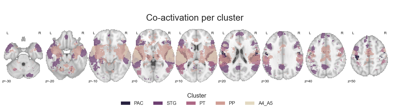
The plot we set up is both informative and clear, coolio. Lets move on to the next analyses: comparing each cluster against the auditory cortex on average.

for image, cluster in zip(contrast_all, cluster_names):
    
    image.to_filename(opj(results_path, 'coactivation-MNI152NLin6Sym_res_02_desc-%sall.nii.gz' %cluster))

Per cluster against entire AC

In the previous step, we contrast each cluster against every other cluster. However, it might also be a good idea to evaluate which voxels and regions co-activate with a given cluster to a greater extent than the auditory cortex on average in order to obtain more cluster-specific information. The only thing we need to change from the step before is to define the contrast parameter and set it to joint:

contrast_allVSac = coactivation_contrast(neurosynth_dataset, 
                                         cluster_solution_loaded, regions=[1,2,3,4,5], 
                                         target_thresh=0.05, q = 0.001, contrast='joint')

And we can use our plotting function again to evaluate the co-activation maps:

make_thresholded_slices(contrast_allVSac, cluster_names, colors=cmap_co_sns, title='Co-activation per cluster against AC', title_coord_x=-805, cut_coords=cut_coords, annotate=True)

<nilearn.plotting.displays.ZSlicer at 0x7fa18bc96780>

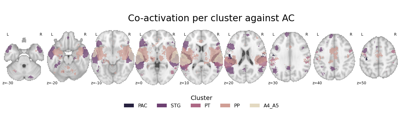
We can definitely see some differences as compared to the previous analyses here.

for image, cluster in zip(contrast_allVSac, cluster_names):
    
    image.to_filename(opj(results_path, 'coactivation-MNI152NLin6Sym_res_02_desc-%sallAC.nii.gz' %cluster))

After these “overview” analyses, it is time to get more into the details here. Thus, within the next analysis steps, we will group the clusters based on the presumptive functional organization of the auditory cortex and subsequently compare them.

Grouped clusters

As mentioned in the manuscript and introduction, prior research suggested that the auditory cortex follows some inherent organizational principles. In more detail, the processing of auditory information is apparently bound to a hierarchical cascade that starts in the primary auditory cortex and progresses towards regions in the superior temporal plane and concludes in the superior temporal gyrus. Notably, this hierarchical processing was observed in both hemispheres and is manifested in two parallel stream, one towards anterior and one towards posterior regions. While all auditory stimuli follow this order, the expression of the respective processing network, specifically the involvement of the left vs. right hemisphere and anterior vs. posterior regions is presumed to diverge as a function of auditory stimulus or category. Based on previous studies on this phenomenon, the spectrotemporal modulations of a given sound can/should be held responsible for this divergence. This refers to the modulations of a given sound along the frequency or spectral domain and the temporal domain, i.e. how much does a sound change with regard to its frequency components within a certain time. Here, the left hemisphere and posterior regions were shown to respond more to/prefer sounds with fast temporal and low spectral modulation such as speech and the right hemisphere and anterior regions sounds with comparably slower temporal and more pronounced spectral modulations such as music. In order to evaluate if this proposed organization is reflected through a corresponding network pattern, the clusters were grouped into sets of clusters based on the introduced hierarchical processing and its diverging expression and their co-activation patterns compared to one another. This entailed the comparison of co-activation patterns between primary and non-primary regions, regions within the STP and regions within the STG, regions in the left and regions in the right hemisphere, as well as anterior and posterior regions. To enable some of the groupings and subsequent comparison, some image operations in terms of accessing distinct single cluster are necessary. Therefore, we will create a function that extracts a given cluster from the cluster solution and returns a new image that only contains the requested cluster. To make things easy to evaluate, we will also include some plotting functionality that will display the extracted cluster its respective color (from the cluster solution).

def get_cluster(cluster_image, region_id, region_name):
    
    cluster_solution_loaded_tmp = deepcopy(cluster_image.get_fdata())
    cluster_solution_loaded_tmp[cluster_solution_loaded_tmp != np.unique(cluster_solution_loaded_tmp)[region_id]] = 0
    cluster_solution_loaded_tmp_img = nb.Nifti1Image(cluster_solution_loaded_tmp, affine=cluster_image.affine)
        
    color_tmp = sns.cubehelix_palette(5, start=-.2, rot=.6, reverse=True).as_hex()[region_id-1]

    import warnings
    warnings.filterwarnings("ignore")

    sns.set_style('white')
    plt.rcParams["font.family"] = "Arial"   

    fig=plt.figure(num=None, figsize=(12, 6))
    check_mask = plot_anat(cut_coords=[-55, -34, 7], figure=fig, draw_cross=False)
    check_mask.add_contours(cluster_solution_loaded_tmp_img, 
                            levels=[0], colors=color_tmp, filled=True)

    plt.text(-205, 90, '%s cluster' %region_name, fontsize=30)

    return cluster_solution_loaded_tmp_img

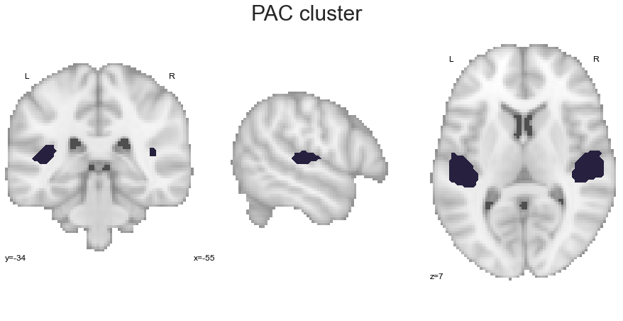
Via employing this function, we can now extract the given clusters one by one, utilizing their respective names that were assigned in the clustering analyses. Please not, that within this first set of grouped co-activation analyses we will not differentiate between hemisphere, thus a given cluster will be present in both. Lets start with the PAC:

PAC_cluster = get_cluster(cluster_solution_loaded, 1, 'PAC')

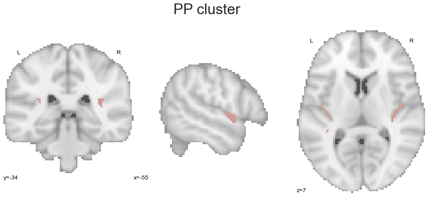
We continue with the PP:

PP_cluster = get_cluster(cluster_solution_loaded, 4, 'PP')

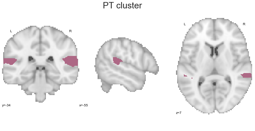
Now the PT:

PT_cluster = get_cluster(cluster_solution_loaded, 3, 'PT')

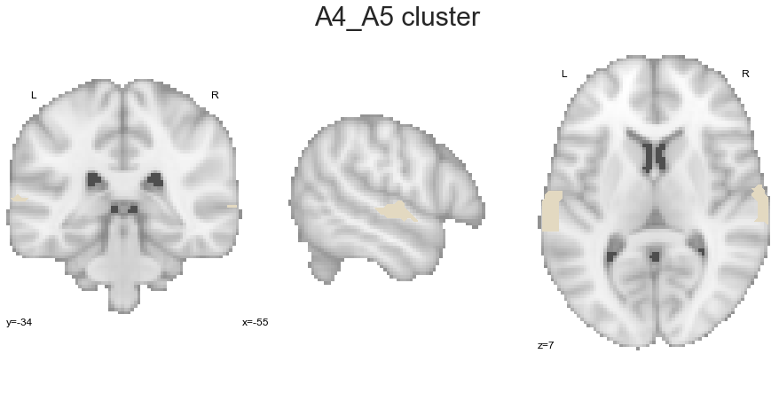
We are leaving the STP and continue with the A4_A5 cluster:

A4_A5_cluster = get_cluster(cluster_solution_loaded, 5, 'A4_A5')

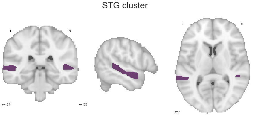
And last but not least, the STG:

STG_cluster = get_cluster(cluster_solution_loaded, 2, 'STG')

With that, we have extract all clusters of our solution. As some comparisons between cluster-specific co-activation patterns can also be conducted directly on our cluster solution, we are going to define the names of clusters and their respective label values:

PAC = 1
PP = 4
PT = 3
A4_A5 = 5
STG = 2

Great, now we can begin with the actual grouped co-activation pattern analyses. As the respective groupings and comparisons require different prerequisites and steps, all of them will vary a bit and there will not be a general function that performs everything. However, each analysis and its steps will of course be explained in detail.

Primary auditory cortex vs. remaining auditory cortex

The first grouping and comparison will focus on the difference between the primary and non-primary auditory cortex. As we already have the primary auditory cortex via the PAC cluster, we only need to gather the remaining clusters into one image. We can use nilearn’s math_img function for that and given that we only want to combine clusters into one image, this is as easy as:

AC_nonprimary = math_img("img1+img2+img3+img4", img1=PP_cluster, img2=PT_cluster,
                         img3=A4_A5_cluster, img4=STG_cluster)

As the clusters still have their original values:

np.unique(AC_nonprimary.get_fdata())

array([0., 2., 3., 4., 5.])

we need to adapt the image so that we can perform the contrast with the PAC cluster. In more detail, we need to set all non-zero voxels (our clusters) to the same value that should be distinct from the PAC cluster. Regarding the latter, it should have only the value 1 for non-zero voxels:

np.unique(PAC_cluster.get_fdata())

array([0., 1.])

Great, that checks out. In order to keep things simple, lets just set the values in the non-primary auditory cortex to 2. A straightforward combination of nibabel and numpy will get us there in no time. At first we get the data of our non-primary auditory cortex image and set all non-zero voxels to 2:

AC_nonprimary_data = AC_nonprimary.get_fdata()
AC_nonprimary_data[AC_nonprimary.get_fdata() > 0] = 2

From this new array, we then create a new image, overwriting the original non-primary auditory cortex image and using its affine:

AC_nonprimary = nb.Nifti1Image(AC_nonprimary_data, affine=AC_nonprimary.affine)

As we now have the clusters we want, we can once again use nilearn’s math_img to combine them into one image that we can then submit to the function that performs the co-activation contrast:

PAC_AC_nonprimary = math_img("img1+img2", img1=PAC_cluster, img2=AC_nonprimary)

However, it is always a good idea to check if things worked out as expected. Thus, let’s plot the resulting image. This also brings up a great and important question: how should clusters be colored now that they are grouped? The PAC cluster can obviously keep its color, but what should be done for the non-primary auditory cortex? To avoid incorporating a new colormap and reflect the corresponding information, we will just take the mean RGB value across all respective clusters:

AC_nonprimary_color = [(STG_color + PT_color + PP_color + A4_A5_color) / 4 for STG_color, PT_color, PP_color, A4_A5_color in 
                       zip(cmap_co_list(1)[:-1], cmap_co_list(2)[:-1], cmap_co_list(3)[:-1], cmap_co_list(4)[:-1])]

Using matplotlib and seaborn we can now combine the resulting color with the PAC cluster color to create both, a ListedColormap and a standard colormap:

PAC_AC_nonprimary_cmap_list = ListedColormap([cmap_co_list(0)[:-1], tuple(AC_nonprimary_color)])
PAC_AC_nonprimary_cmap = sns.color_palette([cmap_co_list(0)[:-1], tuple(AC_nonprimary_color)])

Now, we can plot the primary-vs-non-primary auditory cortex cluster image:

sns.set_style('white')
plt.rcParams["font.family"] = "Arial"   

fig=plt.figure(num=None, figsize=(12, 6))
plot_roi(PAC_AC_nonprimary, cut_coords=[-55, -34, 7], figure=fig, 
         draw_cross=False, cmap=PAC_AC_nonprimary_cmap_list, colorbar=False)

legend_elements = [Patch(facecolor=PAC_AC_nonprimary_cmap_list(0), label='PAC'),
                   Patch(facecolor=PAC_AC_nonprimary_cmap_list(1), label='non-primary AC')]

plt.legend(handles=legend_elements, loc='lower center', bbox_to_anchor=(-0.65, -0.2), 
           frameon=False, ncol=5, title='Clusters', prop={'size': 16}, title_fontsize=20)

plt.text(-320, 90, 'Primary vs. non-primary auditory cortex cluster', fontsize=30)

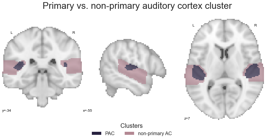
Nice, that looks about right. Having everything in place, we can submit the image to the coactivation_contrast function and as we only have two distinct clusters, we do not need to specify which to compare:

contrast_primaryVSall = coactivation_contrast(neurosynth_dataset, 
                                              PAC_AC_nonprimary,
                                              target_thresh=0.05, q = 0.001)

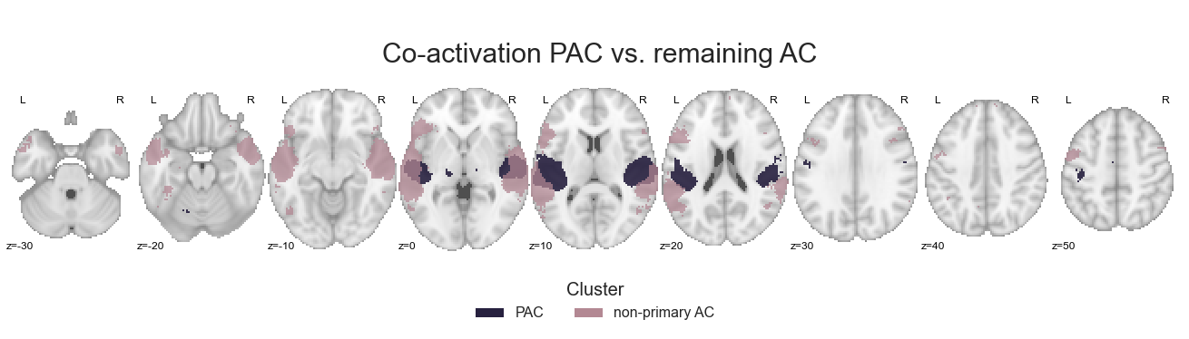
We can investigate the results, that is how co-activation patterns diverge between primary and non-primary auditory cortex using the make_threshold_slices function:

make_thresholded_slices(contrast_primaryVSall, ['PAC', 'non-primary AC'], colors=PAC_AC_nonprimary_cmap, title='Co-activation PAC vs. remaining AC', 
                        title_coord_x=-800, cut_coords=cut_coords, annotate=True)

<nilearn.plotting.displays.ZSlicer at 0x7fa0f7144f28>

Of course, we will also save the results in dedicated images:

for image, cluster in zip(contrast_primaryVSall, ['PAC', 'npAC']):
    
    image.to_filename(opj(results_path, 'coactivation-MNI152NLin6Sym_res_02_desc-%spacVSac.nii.gz' %cluster))

As mentioned above, all grouping anlyses will require different steps. However, the rough outline will be comparable to the one we just performed: create the grouped clusters, create a respective colormap, perform the co-activation analysis and save the results. With that in mind, we will continue with the grouping of STP and STG clusters.

STP vs. STG

In order to provide as much insights as possible, we will not only compare STP to STG clusters, but also clusters within those groupings, i.e. PAC, PP and PT within the STP and A4_A5 and STG within the STG. So lets start with that. At first, the STP: we will use math_img to combine STP clusters within one image:

STP = math_img("img1+img2+img3", img1=PAC_cluster, img2=PT_cluster, img3=PP_cluster)

and as we want to compare them, we do not have to reset their values for now, but can directly check the image (after creating the colormap):

STP_cmap_list = ListedColormap([cmap_co_list(0)[:-1], (1,1,1), cmap_co_list(2)[:-1], cmap_co_list(3)[:-1]])
STP_cmap = sns.color_palette([cmap_co_list(0)[:-1], cmap_co_list(2)[:-1], cmap_co_list(3)[:-1]])

sns.set_style('white')
plt.rcParams["font.family"] = "Arial"   

fig=plt.figure(num=None, figsize=(12, 6))
plot_roi(STP, cut_coords=[-55, -34, 7], figure=fig, 
         draw_cross=False, cmap=STP_cmap_list, colorbar=False)

legend_elements = [Patch(facecolor=STP_cmap_list(0), label='PAC'),
                   Patch(facecolor=STP_cmap_list(2), label='PT'),
                   Patch(facecolor=STP_cmap_list(3), label='PP')]

plt.legend(handles=legend_elements, loc='lower center', bbox_to_anchor=(-0.65, -0.2), 
           frameon=False, ncol=5, title='Clusters', prop={'size': 16}, title_fontsize=20)

plt.text(-210, 90, 'STP clusters', fontsize=30)

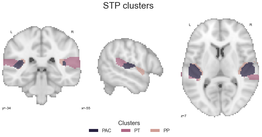
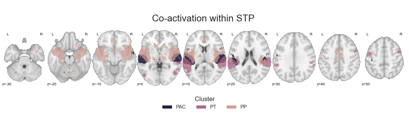
As everything looks ok, we can run the coactivation_contrast function:

contrast_STP = coactivation_contrast(neurosynth_dataset, 
                                     cluster_solution, regions=[1,3,4],
                                     target_thresh=0.05, q = 0.001)

and check the outcomes:

make_thresholded_slices(contrast_STP, ['PAC', 'PT', 'PP'], colors=STP_cmap, title='Co-activation within STP', title_coord_x=-735, cut_coords=cut_coords, annotate=True)

<nilearn.plotting.displays.ZSlicer at 0x7fa0f7510b70>

As before, we will save the cluster-specific co-activation maps:

for image, cluster in zip(contrast_STP, ['PAC', 'PT', 'PP']):
    
    image.to_filename(opj(results_path, 'coactivation-MNI152NLin6Sym_res_02_desc-%sstp.nii.gz' %cluster))

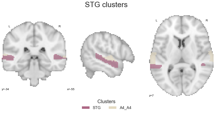
Next up is basically the same for the STG clusters. At first, the STG clusters are combined into one image:

STG = math_img("img1+img2", img1=STG_cluster, img2=A4_A5_cluster)

and after creating the corresponding colormap:

STG_cmap_list = ListedColormap([cmap_co_list(2)[:-1], cmap_co_list(5)[:-1]])
STG_cmap = sns.color_palette([cmap_co_list(2)[:-1], cmap_co_list(5)[:-1]])

are plotted for visual inspection:

sns.set_style('white')
plt.rcParams["font.family"] = "Arial"   

fig=plt.figure(num=None, figsize=(12, 6))
plot_roi(STG, cut_coords=[-55, -34, 7], figure=fig, 
         draw_cross=False, cmap=STG_cmap_list, colorbar=False)

legend_elements = [Patch(facecolor=STG_cmap_list(0), label='STG'),
                   Patch(facecolor=STG_cmap_list(1), label='A4_A4')]

plt.legend(handles=legend_elements, loc='lower center', bbox_to_anchor=(-0.65, -0.2), 
           frameon=False, ncol=5, title='Clusters', prop={'size': 16}, title_fontsize=20)

plt.text(-210, 90, 'STG clusters', fontsize=30)

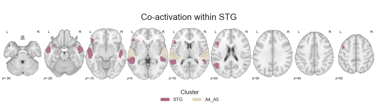
No surprise: we use the coactivation_contrast function to compute and compare co-activation patterns:

contrast_STG = coactivation_contrast(neurosynth_dataset, 
                                     cluster_solution, regions=[2,5],
                                     target_thresh=0.05, q = 0.001)

and check the results:

make_thresholded_slices(contrast_STG, ['STG', 'A4_A5'], colors=STG_cmap, title='Co-activation within STG', title_coord_x=-735, cut_coords=cut_coords, annotate=True)

<nilearn.plotting.displays.ZSlicer at 0x7fa0fc60bac8>

as well as save the obtained co-activation images per cluster:

for image, cluster in zip(contrast_STG, ['STG', 'A4_A5']):
    
    image.to_filename(opj(results_path, 'coactivation-MNI152NLin6Sym_res_02_desc-%sstg.nii.gz' %cluster))

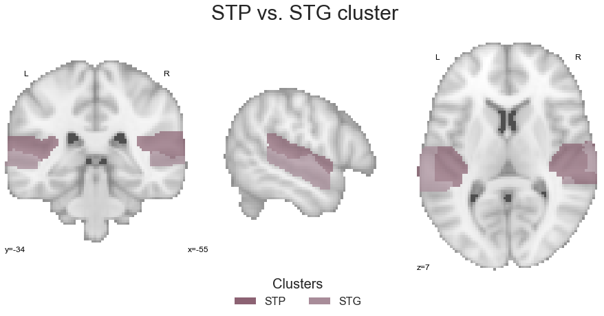
In order to actually compare STP and STG co-activation-patterns, we have to reset the respective cluster values correspondingly and create a new image, combining the resulting grouped cluster images. However, we can do that using the same steps we employed above. At first, we set all non-zero voxels in the STP cluster image to 1:

STP_data = STP.get_fdata()
STP_data[STP.get_fdata() > 0] = 1
STP = nb.Nifti1Image(STP_data, affine=STP.affine)

Second, we do the same for the STG cluster image, but setting non-zero voxels to 2:

STG_data = STG.get_fdata()
STG_data[STG.get_fdata() > 0] = 2
STG = nb.Nifti1Image(STG_data, affine=STG.affine)

As usual by now, we have to create a fitting colormap:

STP_color = [(PAC_color + PT_color + PP_color) / 3 for PAC_color, PT_color, PP_color in zip(cmap_co_list(0)[:-1], cmap_co_list(2)[:-1], cmap_co_list(3)[:-1])]
STG_color = [(STG_color + A4_A5_color ) / 2 for STG_color, A4_A5_color in zip(cmap_co_list(1)[:-1], cmap_co_list(4)[:-1])]
STP_STG_cmap_list = ListedColormap([tuple(STP_color), tuple(STG_color)])
STP_STG_cmap = sns.color_palette([tuple(STP_color), tuple(STG_color)])

And last but not least, we combine them into one image:

STP_STG = math_img("img1+img2", img1=STP, img2=STG)

check the created image:

sns.set_style('white')
plt.rcParams["font.family"] = "Arial"   

fig=plt.figure(num=None, figsize=(12, 6))
plot_roi(STP_STG, cut_coords=[-55, -34, 7], figure=fig, 
         draw_cross=False, cmap=STP_STG_cmap_list, colorbar=False)

legend_elements = [Patch(facecolor=STP_STG_cmap_list(0), label='STP'),
                   Patch(facecolor=STP_STG_cmap_list(1), label='STG')]

plt.legend(handles=legend_elements, loc='lower center', bbox_to_anchor=(-0.65, -0.2), 
           frameon=False, ncol=5, title='Clusters', prop={'size': 16}, title_fontsize=20)

plt.text(-230, 90, 'STP vs. STG cluster', fontsize=30)

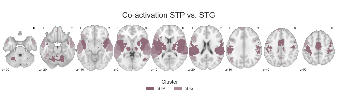
and submit it to the coactivation_contrast function:

contrast_STP_STG = coactivation_contrast(neurosynth_dataset, 
                                         STP_STG, 
                                         target_thresh=0.05, q = 0.001)

Lets plot the results:

make_thresholded_slices(contrast_STP_STG, ['STP', 'STG'], colors=STP_STG_cmap, title='Co-activation STP vs. STG', title_coord_x=-750, cut_coords=cut_coords, annotate=True)

<nilearn.plotting.displays.ZSlicer at 0x7fa0fcfae278>

As with the previous results, we are going to save the grouped cluster-specific co-activation images:

for image, cluster in zip(contrast_STP_STG, ['STP', 'STG']):
    
    image.to_filename(opj(results_path, 'coactivation-MNI152NLin6Sym_res_02_desc-%sstpVSstg.nii.gz' %cluster))

Great! Next up is already the last step within this section of co-activation analyses, the comparison of anterior vs. posterior regions.

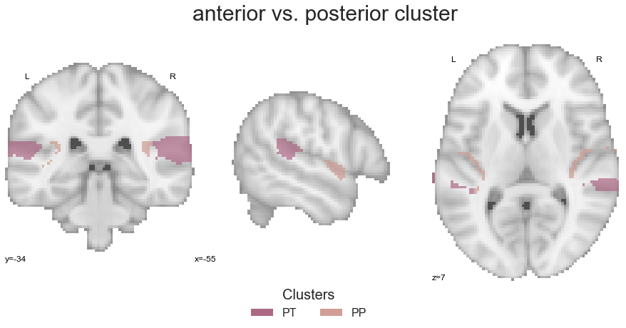
Anterior regions vs. posterior regions

Based on the chosen cluster solution and the spatial distribution of its clusters, the only two that can be utilized to compare anterior and posterior regions are the PT and PP clusters. While it would of course also be interesting to evaluate a potential differentiation in the STG as well, we will keep the data-driven approach and not introduce a manual distinction between e.g. anterior and posterior parts of the STG cluster. Nevertheless, it is obviously something to discuss and think about. For now, we will apply the usual steps to the PT and PP cluster. As it is once again a binary comparison within which we do not have to reset cluster values, we can directly go to the step where we combine the clusters into one image:

ant_post = math_img("img1+img2", img1=PT_cluster, img2=PP_cluster)

The generation of a respective colormap is the same as before:

ant_post_cmap_list = ListedColormap([cmap_co_list(2)[:-1], cmap_co_list(3)[:-1]])
ant_post_cmap = sns.color_palette([cmap_co_list(2)[:-1], cmap_co_list(3)[:-1]])

The same holds true for the evaluation plot:

sns.set_style('white')
plt.rcParams["font.family"] = "Arial"   

fig=plt.figure(num=None, figsize=(12, 6))
plot_roi(ant_post, cut_coords=[-55, -34, 7], figure=fig, 
         draw_cross=False, cmap=ant_post_cmap_list, colorbar=False)

legend_elements = [Patch(facecolor=ant_post_cmap_list(0), label='PT'),
                   Patch(facecolor=ant_post_cmap_list(1), label='PP')]

plt.legend(handles=legend_elements, loc='lower center', bbox_to_anchor=(-0.65, -0.2), 
           frameon=False, ncol=5, title='Clusters', prop={'size': 16}, title_fontsize=20)

plt.text(-250, 90, 'anterior vs. posterior cluster', fontsize=30)

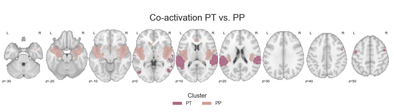
That is it, we can already compute the co-activation patterns:

contrast_ant_post = coactivation_contrast(neurosynth_dataset, 
                                          ant_post, regions=[3,4],
                                          target_thresh=0.05, q = 0.001)

and visualize the results:

make_thresholded_slices(contrast_ant_post, ['PT', 'PP'], colors=ant_post_cmap, title='Co-activation PT vs. PP', title_coord_x=-725, cut_coords=cut_coords, annotate=True)

<nilearn.plotting.displays.ZSlicer at 0x7fa0fe956e80>

After saving the cluster-specific co-activation images:

for image, cluster in zip(contrast_ant_post, ['PT', 'PP']):
    
    image.to_filename(opj(results_path, 'coactivation-MNI152NLin6Sym_res_02_desc-%santVSpost.nii.gz' %cluster))

this section is concluded and we obtained co-activation images for cluster groupings and subsequent comparisons. However, the groupings only entail a subset of the proposed organizational principles of the auditory cortex. The “classic” and most prominent one is so far missing and will be focused on in the next section.

Per cluster between hemisphere

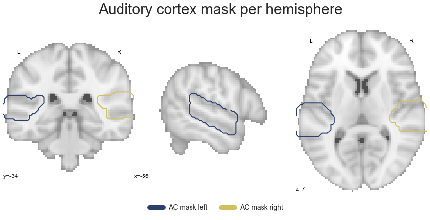
While we already conducted quite a bunch of co-activation analyses, one set for each cluster and one set based on certain groupings, we always utilized the clusters as they included in the chosen cluster solution. In more detail, this refers to bilateral clusters as in every case, clusters are present in both the left and right hemisphere. The thing is: the potential differentiation between the left and right auditory cortex is the basis for the strongest claims concerning its functional organization, i.e. the preferred processing of e.g. speech in the left and music in the right hemisphere. Therefore, we need to gather and subsequently group as well as compare clusters in a hemisphere-specific manner. The first step to make this happen is to extract clusters for each hemisphere. As we not only created a bilateral auditory cortex mask, but also hemisphere-specific ones, we can make use of the latter to achieve this. Initially, we set these masks:

ac_mask_left = opj(ac_roi_path, 'tpl-MNI152NLin6Sym_res_02_desc-ACleftdilated_mask.nii.gz')
ac_mask_right = opj(ac_roi_path, 'tpl-MNI152NLin6Sym_res_02_desc-ACrightdilated_mask.nii.gz')

and check them to make sure everything is as we remember:

sns.set_style('white')
plt.rcParams["font.family"] = "Arial"   

fig=plt.figure(num=None, figsize=(12, 6))
ac_mask_both = plot_anat(cut_coords=[-55, -34, 7], figure=fig, draw_cross=False)
ac_mask_both.add_contours(ac_mask_left, linewidths=2,
                        levels=[0], colors=sns.color_palette('cividis', 5).as_hex()[0])
ac_mask_both.add_contours(ac_mask_right, linewidths=2,
                        levels=[0], colors=sns.color_palette('cividis', 5).as_hex()[4])

roi_legend = [Line2D([0], [0], color=sns.color_palette('cividis', 5)[0], lw=9, label='AC mask left'),
              Line2D([0], [0], color=sns.color_palette('cividis', 5)[4], lw=9, label='AC mask right')]
plt.legend(handles=roi_legend, bbox_to_anchor=(-0.05,-0.1), loc="right", ncol=2,  prop={'size': 14}, frameon=False)


plt.text(-290, 90, 'Auditory cortex mask per hemisphere',
         fontsize=30)

This checks out. As we already have our small get_cluster function that extracts a given cluster across both hemispheres, we can simply extend it to create a new function that does the same, but for each hemisphere:

def get_cluster_hemisphere(cluster, cluster_name=None):
    
    ac_masker_left = NiftiMasker(mask_img=ac_mask_left)
    ac_masker_right = NiftiMasker(mask_img=ac_mask_right)
    
    tmp_left = ac_masker_left.fit_transform(cluster).squeeze()
    tmp_right = ac_masker_right.fit_transform(cluster).squeeze()
    
    tmp_left = ac_masker_left.inverse_transform(tmp_left)
    tmp_right = ac_masker_right.inverse_transform(tmp_right)
    
    sns.set_style('white')
    plt.rcParams["font.family"] = "Arial"   

    fig=plt.figure(num=None, figsize=(12, 6))
    ac_mask_both = plot_anat(cut_coords=[-55, -34, 7], figure=fig, draw_cross=False)
    ac_mask_both.add_contours(tmp_left, linewidths=2, filled=True,
                              levels=[0], colors=sns.color_palette('cividis', 5).as_hex()[0])
    ac_mask_both.add_contours(tmp_right, linewidths=2, filled=True,
                              levels=[0], colors=sns.color_palette('cividis', 5).as_hex()[4])

    if cluster_name is None:
        print("Please provide the name of the cluster.")
    else:
        roi_legend = [Line2D([0], [0], color=sns.color_palette('cividis', 5)[0], lw=9, label='%s cluster left' %cluster_name),
                      Line2D([0], [0], color=sns.color_palette('cividis', 5)[4], lw=9, label='%s cluster right' %cluster_name)]
        plt.legend(handles=roi_legend, bbox_to_anchor=(0.1,-0.1), loc="right", ncol=2,  prop={'size': 14}, frameon=False)


        plt.text(-255, 90, '%s cluster per hemisphere' %cluster_name, fontsize=30)
        
        tmp_left.to_filename(opj(cluster_path, 'tpl-MNI152NLin6Sym_atlas-nsac_desc-5%sleft.nii.gz' %cluster_name))
        tmp_right.to_filename(opj(cluster_path, 'tpl-MNI152NLin6Sym_atlas-nsac_desc-5%sright.nii.gz' %cluster_name))  
        
    return tmp_left, tmp_right

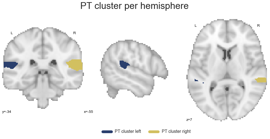
and repeat the steps from above, obtaining hemisphere-specific clusters. We are going to start with the PAC cluster again:

PAC_cluster_left, PAC_cluster_right = get_cluster_hemisphere(PAC_cluster, cluster_name='PAC') 

Next in line is the PT cluster:

PT_cluster_left, PT_cluster_right = get_cluster_hemisphere(PT_cluster, cluster_name='PT') 

The last cluster in the STP is the PP:

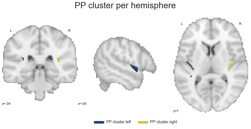
PP_cluster_left, PP_cluster_right = get_cluster_hemisphere(PP_cluster, cluster_name='PP') 

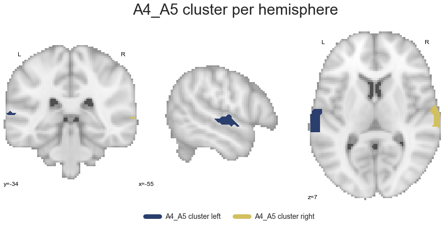
Going further down the processing stream, we extract the A4_A5 cluster:

A4_A5_cluster_left, A4_A5_cluster_right = get_cluster_hemisphere(A4_A5_cluster, cluster_name='A4_A5') 

and finally the STG cluster:

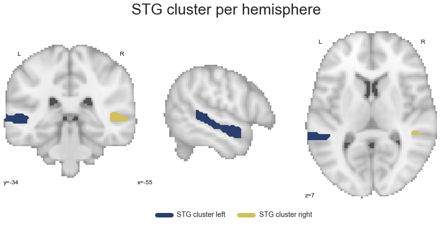
STG_cluster_left, STG_cluster_right = get_cluster_hemisphere(STG_cluster, cluster_name='STG') 

Now that we have all clusters in a hemisphere-specific manner, we can continue with the co-activation analyses based on respective groupings.

Left vs. right auditory cortex

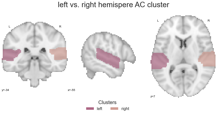
Going once more from a broad overview to more specific analyses, we will start by grouping and subsequently comparing the left and right auditory cortex as a whole. To this end, we will create a left hemisphere auditory cortex image and a right hemisphere auditory cortex image utilizing the same approach as we did before. Lets start with the left hemisphere:

left_hemisphere = math_img("img1+img2+img3+img4+img5", img1=PAC_cluster_left, img2=PP_cluster_left, 
                           img3=PT_cluster_left, img4=A4_A5_cluster_left, img5=STG_cluster_left)

We do the same for the right hemisphere:

right_hemisphere = math_img("img1+img2+img3+img4+img5", img1=PAC_cluster_right, img2=PP_cluster_right, 
                           img3=PT_cluster_right, img4=A4_A5_cluster_right, img5=STG_cluster_right)

Given that all analyses within this section are going to be binary ones, we will define a small function that resets all no-zero voxels in the left hemisphere to 1 and all no-zero voxels in the right hemisphere to 2:

def reset_cluster_values(cluster_left, cluster_right):
    
    cluster_left.get_data()[cluster_left.get_data().nonzero()] = 1
    cluster_right.get_data()[cluster_right.get_data().nonzero()] = 2  

Lets put this function to work:

reset_cluster_values(left_hemisphere, right_hemisphere)

We can now combine the left and right hemisphere auditory cortex images into one:

left_right_hemisphere = math_img("img1+img2", img1=left_hemisphere, img2=right_hemisphere)

define a colormap:

hem_cmap_list = ListedColormap([cmap_co_list(2)[:-1], cmap_co_list(3)[:-1]])
hem_cmap = sns.color_palette([cmap_co_list(2)[:-1], cmap_co_list(3)[:-1]])

and after a brief evaluation:

sns.set_style('white')
plt.rcParams["font.family"] = "Arial"   

fig=plt.figure(num=None, figsize=(12, 6))
plot_roi(left_right_hemisphere, cut_coords=[-55, -34, 7], figure=fig, 
         draw_cross=False, cmap=ant_post_cmap_list, colorbar=False)

legend_elements = [Patch(facecolor=hem_cmap_list(0), label='left'),
                   Patch(facecolor=hem_cmap_list(1), label='right')]

plt.legend(handles=legend_elements, loc='lower center', bbox_to_anchor=(-0.65, -0.2), 
           frameon=False, ncol=5, title='Clusters', prop={'size': 16}, title_fontsize=20)

plt.text(-270, 90, 'left vs. right hemispere AC cluster', fontsize=30)

submit it to the coactivation_contrast function:

contrast_left_right = coactivation_contrast(neurosynth_dataset, 
                                            left_right_hemisphere, 
                                            target_thresh=0.05, q = 0.001)

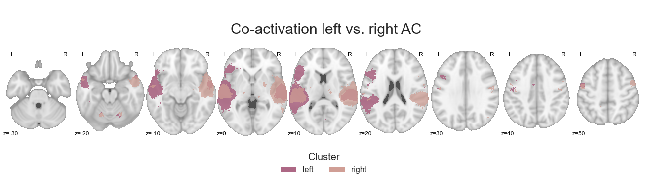
Are there any prominent differences in left vs. right co-activation patterns? Lets find out:

make_thresholded_slices(contrast_left_right, ['left', 'right'], colors=hem_cmap, title='Co-activation left vs. right AC', title_coord_x=-755, cut_coords=cut_coords, annotate=True)

<nilearn.plotting.displays.ZSlicer at 0x7fa0f8f09710>

One thing left to do: saving the respective co-activation maps.

for image, cluster in zip(contrast_left_right, ['left', 'right']):
    
    image.to_filename(opj(results_path, 'coactivation-MNI152NLin6Sym_res_02_desc-%slhacVSrhac.nii.gz' %cluster))

After this rather holistic and broad comparison of hemisphere-specific co-activation patterns, it’s time to go more into detail by contrasting distinct clusters.

Left vs. right hemisphere for each cluster

Comparable to the previous step, we will now compare the co-activation pattern of each cluster between the left and right hemisphere. As we have already extracted the clusters per hemisphere and have our small function to reset the respective values for the binary comparison, this is straightforward. We will start with the PAC.

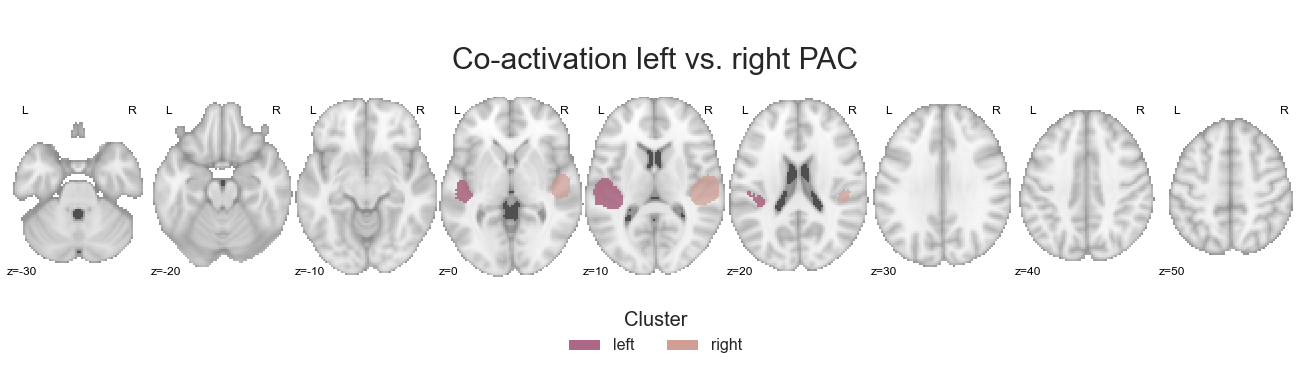
Left vs. right hemisphere for each cluster - PAC

At, first we reset the cluster values so that the left PAC has a value of 1 and the right PAC a value of 2.

reset_cluster_values(PAC_cluster_left, PAC_cluster_right)

We combine both into one image:

left_right_PAC = math_img("img1+img2", img1=PAC_cluster_left, img2=PAC_cluster_right)

and submit the outcome to the coactivation_contrast function:

contrast_left_right_PAC = coactivation_contrast(neurosynth_dataset, 
                                                left_right_PAC,
                                                target_thresh=0.05, q = 0.001)

Using the make_thresholded_slices function we can then visualize the results as done throughout this section:

make_thresholded_slices(contrast_left_right_PAC, ['left', 'right'], colors=hem_cmap, title='Co-activation left vs. right PAC', title_coord_x=-770, cut_coords=cut_coords, annotate=True)

<nilearn.plotting.displays.ZSlicer at 0x7fa0f0b3ef28>

We will of course also save the co-activation maps:

for image, cluster in zip(contrast_left_right_PAC, ['left', 'right']):
    
    image.to_filename(opj(results_path, 'coactivation-MNI152NLin6Sym_res_02_desc-%slhpacVSrhpac.nii.gz' %cluster))

As just said: no problemo at all, given that we have everything in place. Let’s check out the next cluster.

Left vs. right hemisphere for each cluster - PT

How do the co-activation patterns of the PT cluster compare between the hemispheres? To find that out, we reset the cluster values:

reset_cluster_values(PT_cluster_left, PT_cluster_right)

combine the left and the right PT into one image:

left_right_PT = math_img("img1+img2", img1=PT_cluster_left, img2=PT_cluster_right)

and provide that as input to our coactivation_contrast function:

contrast_left_right_PT = coactivation_contrast(neurosynth_dataset, 
                                               left_right_PT, 
                                               target_thresh=0.05, q = 0.001)

It’s time to check the results:

make_thresholded_slices(contrast_left_right_PT, ['left', 'right'], colors=hem_cmap, title='Co-activation left vs. right PT', title_coord_x=-765, cut_coords=cut_coords, annotate=True)

<nilearn.plotting.displays.ZSlicer at 0x7fa0ef9ff828>

As usual, we’ll save the maps:

for image, cluster in zip(contrast_left_right_PT, ['left', 'right']):
    
    image.to_filename(opj(results_path, 'coactivation-MNI152NLin6Sym_res_02_desc-%slhptVSrhpt.nii.gz' %cluster))

Thinking about comprehensive functions and workflows really pays off, doesn’t it?

Left vs. right hemisphere for each cluster - PT

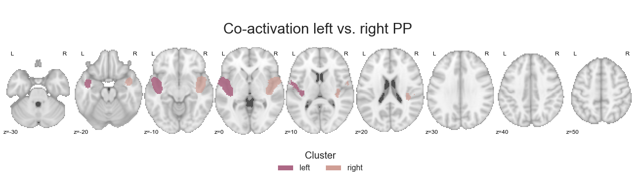
Next up is the PP cluster. The reset_cluster_values function will reset the cluster value in the left hemisphere to 1 and in the right hemisphere to 2.

reset_cluster_values(PP_cluster_left, PP_cluster_right)

Using math_img, we combine both:

left_right_PP = math_img("img1+img2", img1=PP_cluster_left, img2=PP_cluster_right)

and via coactivation_contrast, we can compute hemisphere-specific co-activation patterns:

contrast_left_right_PP = coactivation_contrast(neurosynth_dataset, 
                                               left_right_PP, 
                                               target_thresh=0.05, q = 0.001)

Are things strongly lateralized as within the PAC or maybe a bit bilateral as within the PT? Lets find out:

make_thresholded_slices(contrast_left_right_PP, ['left', 'right'], colors=hem_cmap, title='Co-activation left vs. right PP', title_coord_x=-765, cut_coords=cut_coords, annotate=True)

<nilearn.plotting.displays.ZSlicer at 0x7fa0f3866ba8>

The last thing we have to do is saving the respective co-activation maps.

for image, cluster in zip(contrast_left_right_PP, ['left', 'right']):
    
    image.to_filename(opj(results_path, 'coactivation-MNI152NLin6Sym_res_02_desc-%slhppVSrhpp.nii.gz' %cluster))

It’s time to leave the STP and have a look how the hemisphere-specific co-activation patterns of the STG clusters compare to one another.

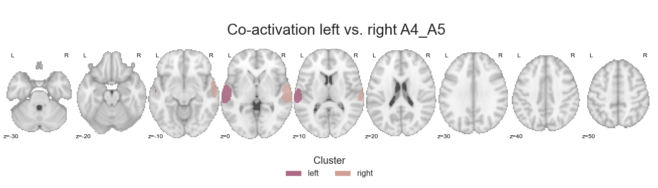
Left vs. right hemisphere for each cluster - A4_A5

At first, we’ll run the analyses for the A4_A5 cluster, starting with resetting the cluster values.

reset_cluster_values(A4_A5_cluster_left, A4_A5_cluster_right)

The clusters are then combined into one image:

left_right_A4_A5 = math_img("img1+img2", img1=A4_A5_cluster_left, img2=A4_A5_cluster_right)

which is utilized to compute the co-activation contrast between them:

contrast_left_right_A4_A5 = coactivation_contrast(neurosynth_dataset, 
                                                  left_right_A4_A5, 
                                                  target_thresh=0.05, q = 0.001)

Hello make_thresholded_slices function, my old friend…

make_thresholded_slices(contrast_left_right_A4_A5, ['left', 'right'], colors=hem_cmap, title='Co-activation left vs. right A4_A5', title_coord_x=-770, cut_coords=cut_coords, annotate=True)

<nilearn.plotting.displays.ZSlicer at 0x7fa0ecc777f0>

We’ll save these co-activation maps:

for image, cluster in zip(contrast_left_right_A4_A5, ['left', 'right']):
    
    image.to_filename(opj(results_path, 'coactivation-MNI152NLin6Sym_res_02_desc-%slha4a5VSrha4a5.nii.gz' %cluster))

and with that already reached the final step, i.e. cluster.

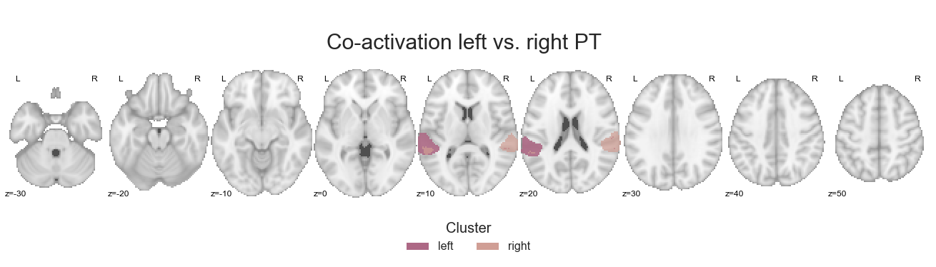
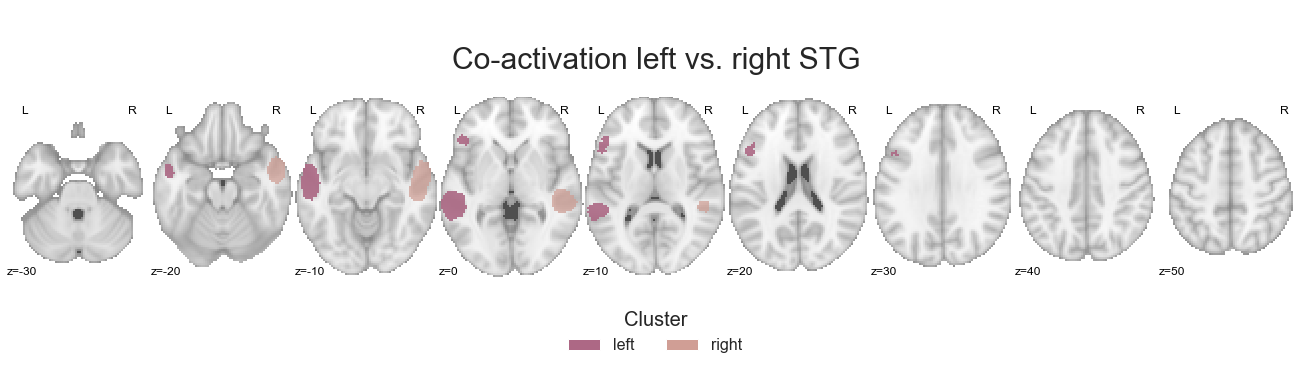
Left vs. right hemisphere for each cluster - STG

In the previous analyses the STG cluster had prominent co-activation with voxels/regions outside the auditory cortex, which seemed to be driven by the left hemisphere. This analysis step should help us clarify this further. Initially, we reset the cluster values:

reset_cluster_values(STG_cluster_left, STG_cluster_right)

and combine both:

left_right_STG = math_img("img1+img2", img1=STG_cluster_left, img2=STG_cluster_right)

One last time, the coactivation_contrast function will compute co-activation patterns:

contrast_left_right_STG = coactivation_contrast(neurosynth_dataset, 
                                                left_right_STG, 
                                                target_thresh=0.05, q = 0.001)

which will be then be plotted via make_thresholded_slices:

make_thresholded_slices(contrast_left_right_STG, ['left', 'right'], colors=hem_cmap, title='Co-activation left vs. right STG', title_coord_x=-770, cut_coords=cut_coords, annotate=True)

<nilearn.plotting.displays.ZSlicer at 0x7fa0eb8d60f0>

and finally saved:

for image, cluster in zip(contrast_left_right_STG, ['left', 'right']):
    
    image.to_filename(opj(results_path, 'coactivation-MNI152NLin6Sym_res_02_desc-%slhstgVSrhstg.nii.gz' %cluster))

This concludes the co-activation analyses of which we did a lot. However, there was also a lot to explore and test!

Summary & outlook