.ipynb .pdf

repository open issue suggest edit

Binder

Contents

Deep learning basics

Peer Herholz (he/him)
Postdoctoral researcher - NeuroDataScience lab at MNI/McGill, UNIQUE
Member - BIDS, ReproNim, Brainhack, Neuromod, OHBM SEA-SIG

  @peerherholz

A brief recap & first overview

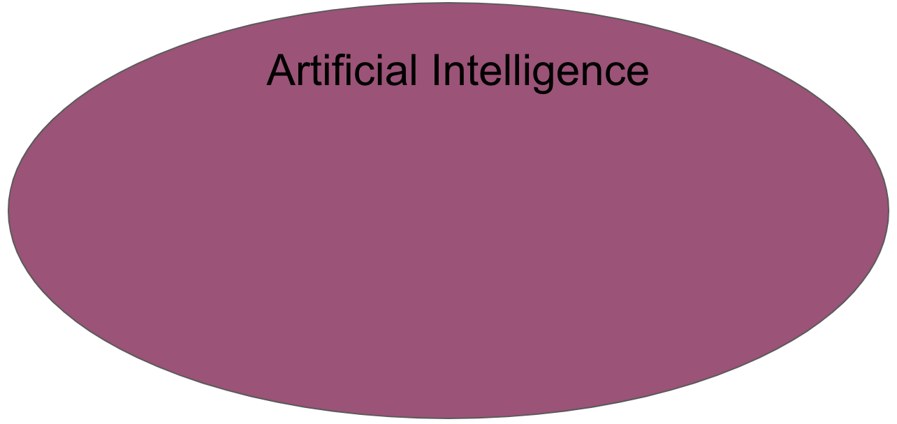
Artificial intelligence (AI) is intelligence demonstrated by machines, as opposed to the natural intelligence displayed by humans or animals. Leading AI textbooks define the field as the study of “intelligent agents”: any system that perceives its environment and takes actions that maximize its chance of achieving its goals. Some popular accounts use the term “artificial intelligence” to describe machines that mimic “cognitive” functions that humans associate with the human mind, such as “learning” and “problem solving”, however this definition is rejected by major AI researchers.

https://en.wikipedia.org/wiki/Artificial_intelligence

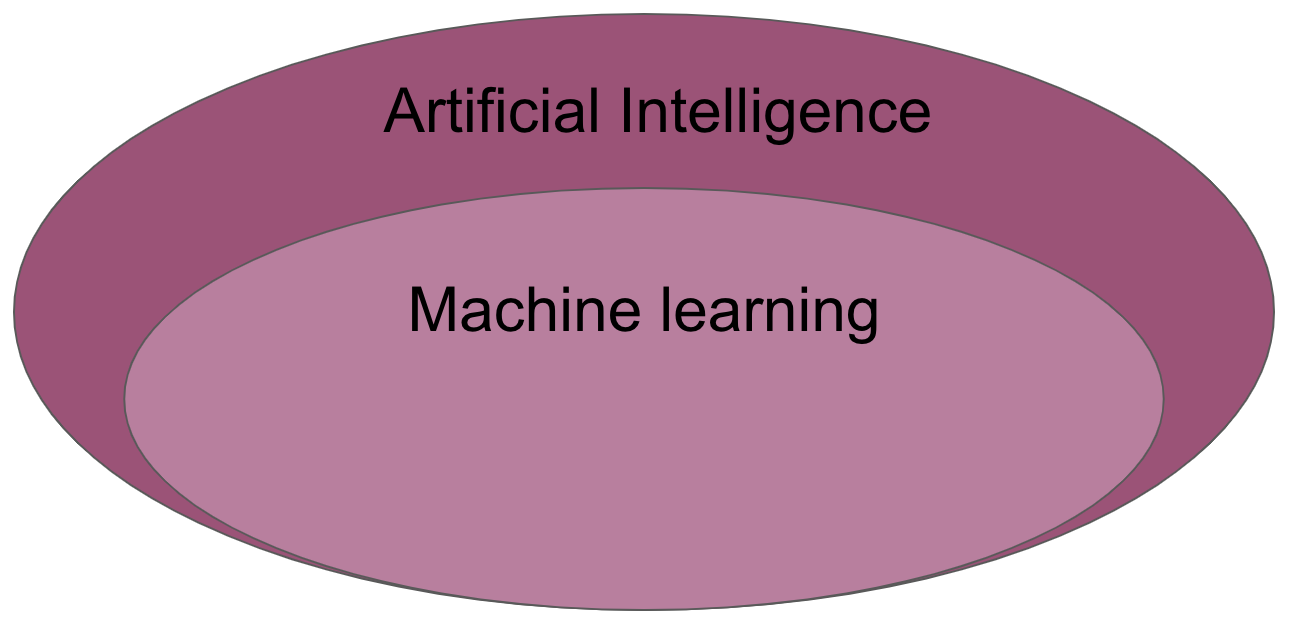
Machine learning (ML) is the study of computer algorithms that can improve automatically through experience and by the use of data. It is seen as a part of artificial intelligence. Machine learning algorithms build a model based on sample data, known as “training data”, in order to make predictions or decisions without being explicitly programmed to do so. A subset of machine learning is closely related to computational statistics, which focuses on making predictions using computers; but not all machine learning is statistical learning. The study of mathematical optimization delivers methods, theory and application domains to the field of machine learning. Data mining is a related field of study, focusing on exploratory data analysis through unsupervised learning. Some implementations of machine learning use data and neural networks in a way that mimics the working of a biological brain.

https://en.wikipedia.org/wiki/Machine_learning

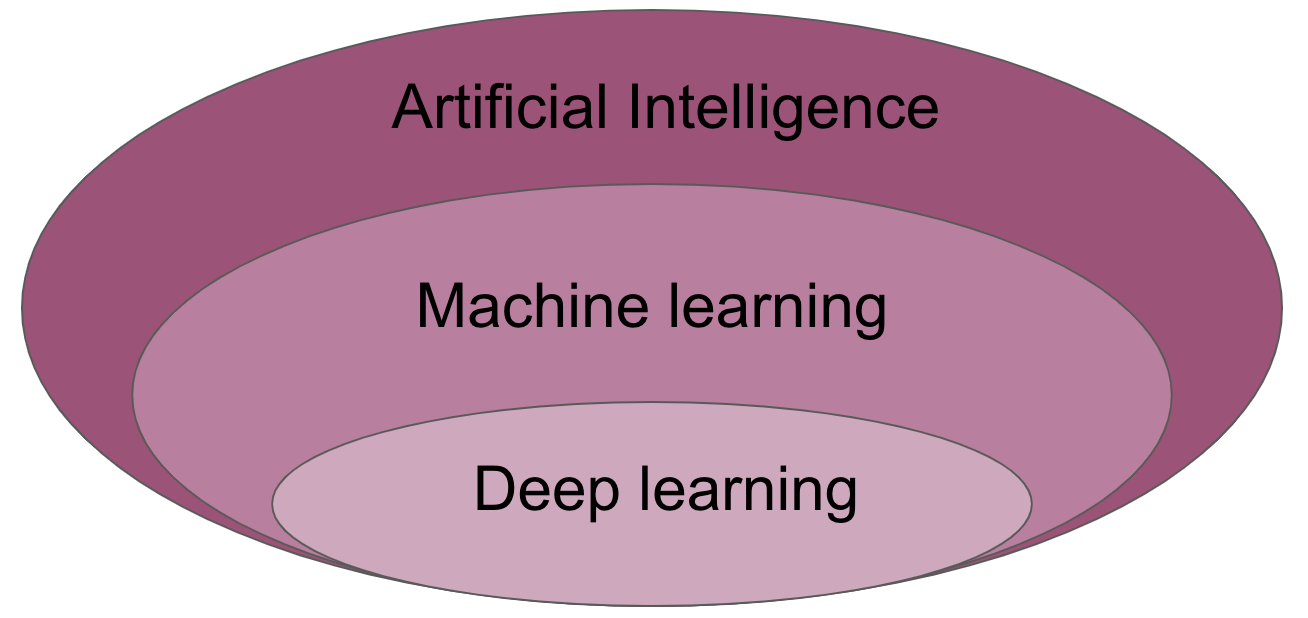
Deep learning (also known as deep structured learning) is part of a broader family of machine learning methods based on artificial neural networks with representation learning. Learning can be supervised, semi-supervised or unsupervised. Artificial neural networks (ANNs) were inspired by information processing and distributed communication nodes in biological systems. ANNs have various differences from biological brains. Specifically, neural networks tend to be static and symbolic, while the biological brain of most living organisms is dynamic (plastic) and analogue. The adjective “deep” in deep learning refers to the use of multiple layers in the network. Early work showed that a linear perceptron cannot be a universal classifier, but that a network with a nonpolynomial activation function with one hidden layer of unbounded width can.

https://en.wikipedia.org/wiki/Deep_learning

• very important: deep learning is machine learning

  • DL is a specific subset of ML

  • structured vs. unstructured input

  • linearity

  • model architectures

• you and “the machine”

  • ML models can become better at a specific task, however they need some form of guidance

  • DL models in contrast require less human intervention

• Why the buzz?

  • works amazing on structured input

  • highly flexible → universal function approximator

• What are the challenges?

  • large number of parameters → data hungry

  • large number of hyper-parameters → difficult to train

• When do I use it?

  • if you have highly-structured input, eg. medical images.

  • you have a lot of data and computational resources.

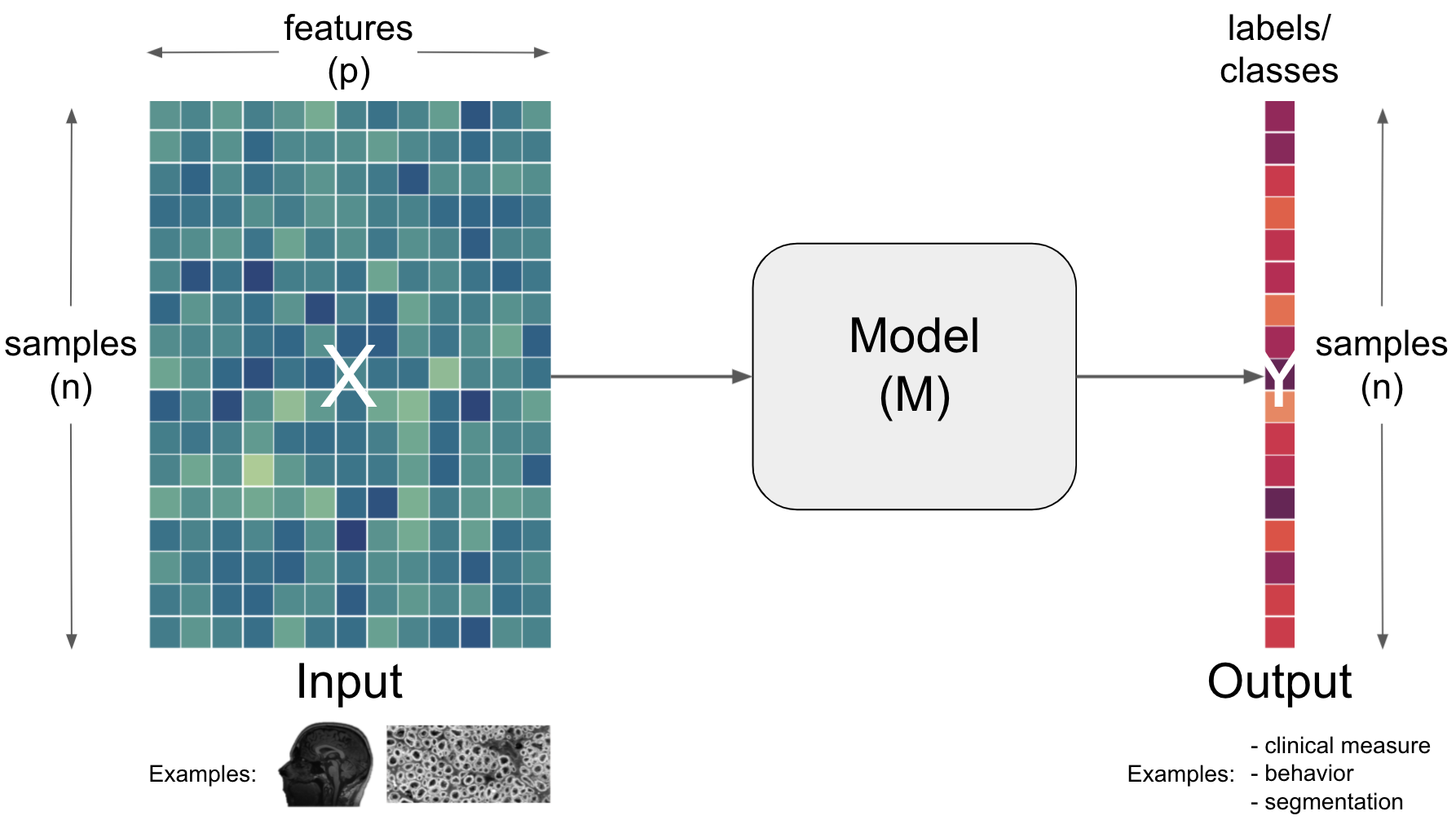
Why go deep learning in neuroscience? (all highly discussed)

• complexity of biological systems

  • integrate knowledge of biological systems in computational systems (excitation vs. inhibition, normalization, LIF)

  • linear-nonlinear processing

  • utilize computational systems as model systems

Why go deep learning in neuroscience? (all highly discussed)

• limitations of “simple models”

  • fail to capture diversity of biological systems (response heterogeneity, sensitivity vs. specificity, etc.)

  • fail to perform as good as biological systems

Why go deep learning in neuroscience? (all highly discussed)

• addressing the “why question”

  • why do biological systems work in the way they do

  • insights into objectives and constraints defined by evolutionary pressure

Aim(s) of this section

• learn about basics behind deep learning, specifically artificial neural networks

• become aware of central building blocks and aspects of artificial neural networks

• get to know different model types and architectures

Outline for this section

1. Deep learning - basics & reasoning

   • learning problems

   • representations

2. From biological to artificial neural networks

   • neurons

   • universal function approximation

3. components of ANNs

   • building parts

   • learning

4. ANN architectures

   • Multilayer perceptrons

   • Convolutional neural networks

Deep learning - basics & reasoning

• as said before: deep learning is (a subset of) machine learning

• it thus includes the core aspects we talked about in the previous section and builds upon them:

  • different learning problems and resulting models/architectures

  • loss function & optimization

  • training, evaluation, validation

  • biases & problems

• this furthermore transfers to the key components you as a user has to think about

  • objective function (What is the goal?)

  • learning rule (How should weights be updated to improve the objective function?)

  • network architecture (What are the network parts and how are they connected?)

  • initialisation (How are weights initially defined?)

  • environment (What kind of data is provided for/during the learning?)

Learning problems

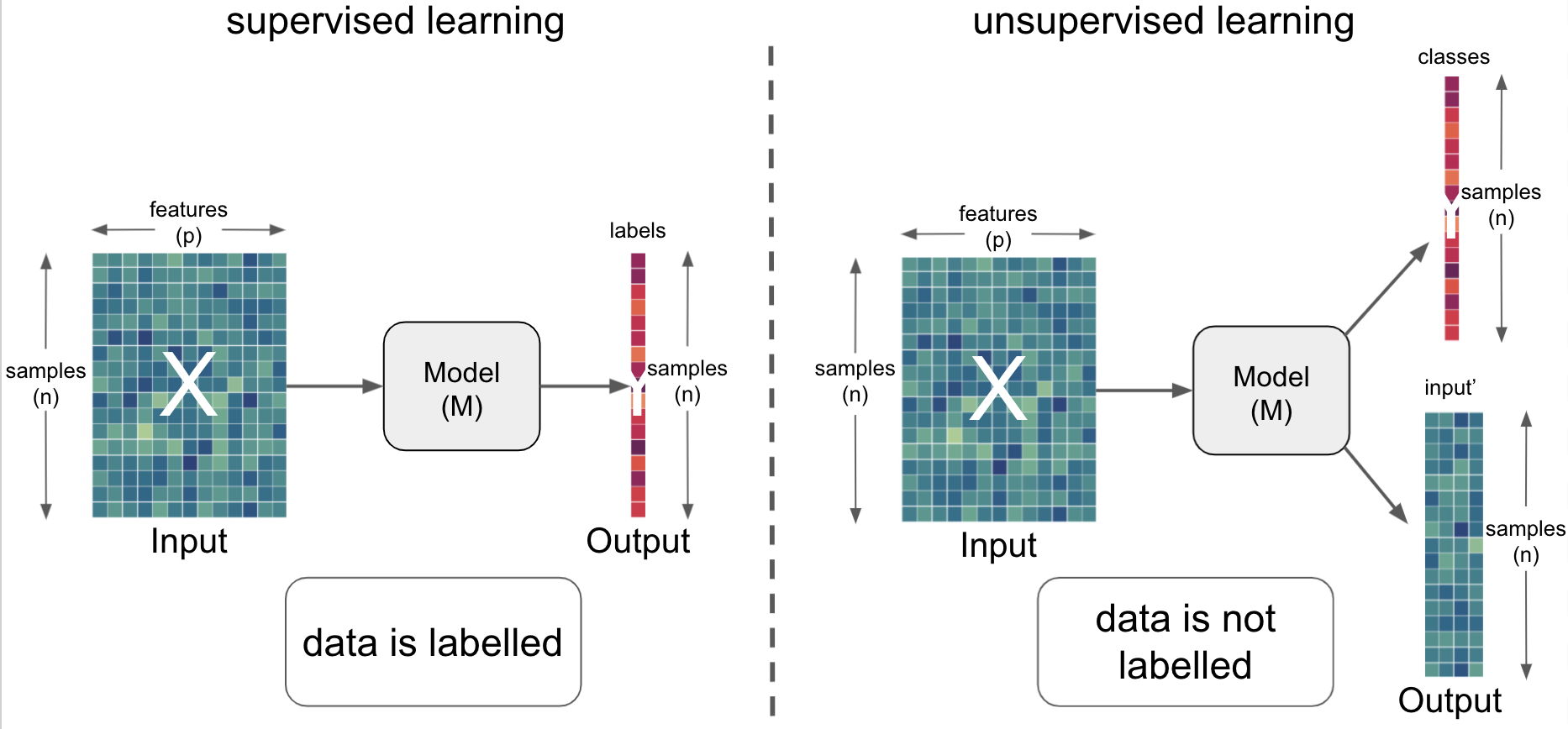
As in machine learning in general, we have supervised & unsupervised learning problems again:

However, within the world of deep learning, we have three more learning problems:

• reinforcement learning

• semi-supervised learning

• self-supervised learning

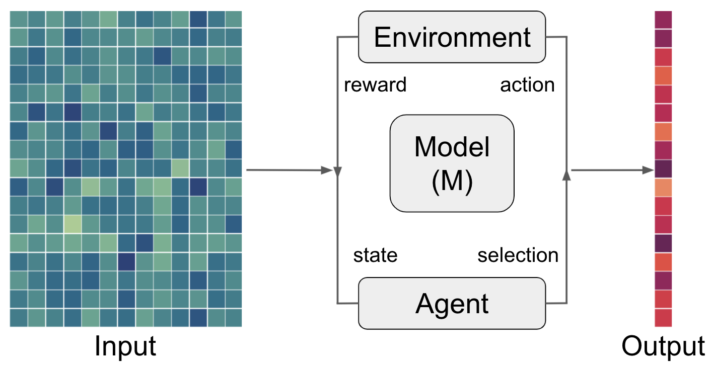
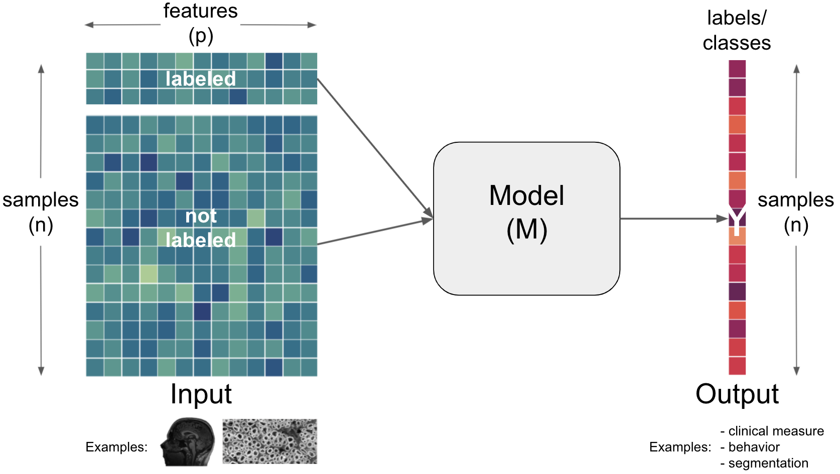
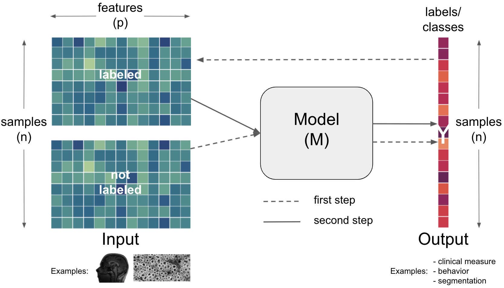
• depending on the data and task, these learning problems can be employed within a diverse set of artificial neural network architectures (most commonly):

  • Multilayer perceptrons

  • Convolutional neural networks

  • Recurrent neural networks

But why employ artificial neural networks at all?

The problem of variance & how representations can help

Think about all the things you as an biological agent do on a typical day … Everything (most things) you do appear very easy to you. Then why is so hard for artificial agents to achieve a comparable behavior and/or performance?

One major problem is the variance of the input we encounter which subsequently makes it very hard to find appropriate transformations that can lead to/help to achieve generalizable behavior.

How about an example? We’ll keep it very simple and focus on recognizing a certain category of the natural world.

You all waited for it and now it’s finally happening: cute cats!

• let’s assume we want to learn to recognize, label and predict “cats” based on a set of images that look like this

• utilizing the models and approaches we talked about so far, we would use predetermined transformations (features) of our data X:

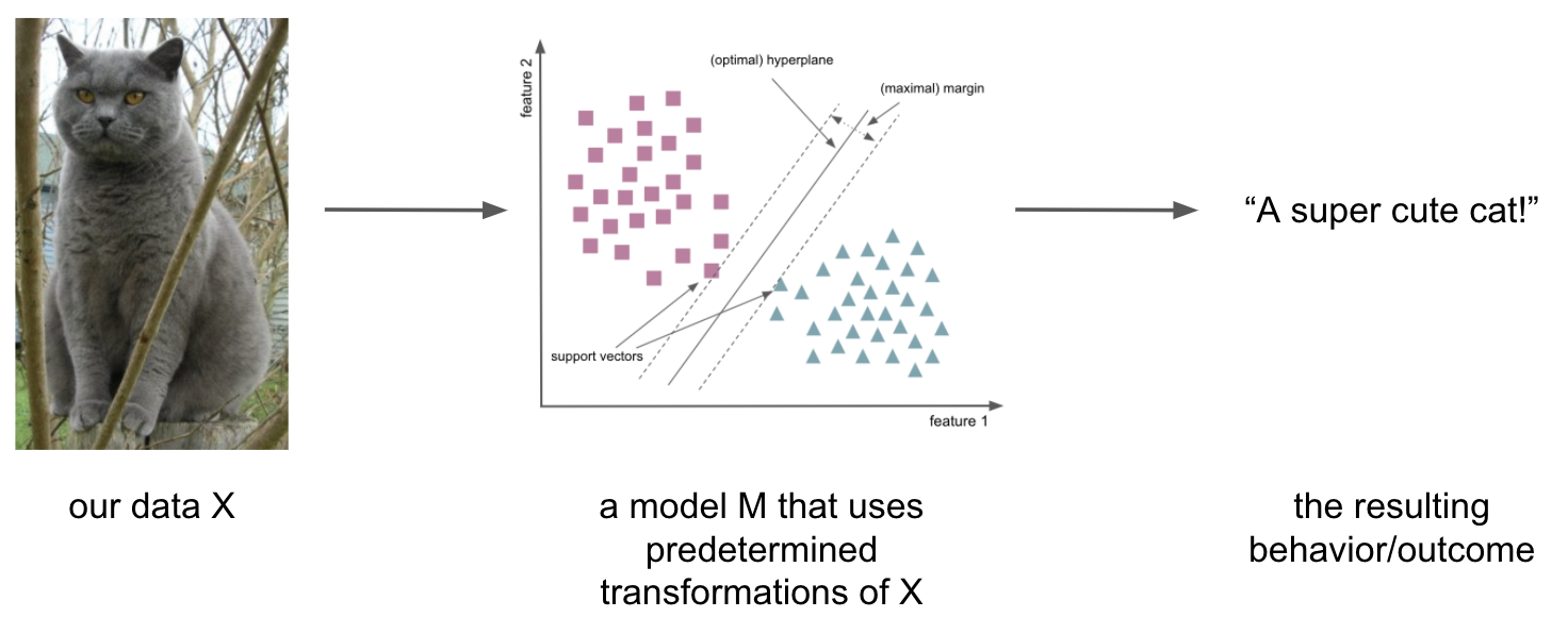
• this constitutes a form of inductive bias, i.e. assumptions we include in the learning problem and thus back into the respective models

• however, this is by far not the only way we could encounter a cat … there are a lots of sources of variation of our data X, including:

• illumination

• deformation

• occlusion

• background clutter

• and intraclass variation

• these variations (and many more) are usually not accounted for and our mapping from X to Y would fail

• what we want to learn to prevent this are invariant representations that capture latent variables which are variables you (most likely) cannot directly observe, but that affect the variables you can observe

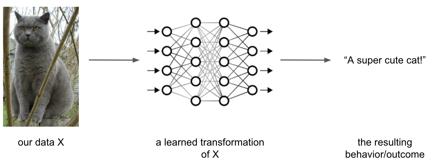
• the “simple models” we talked about so far work with predetermined transformations and thus perform shallow learning, more “complex models” perform deep learning in their hidden layers to learn representations

_{^{https://media1.giphy.com/media/26ufdipQqU2lhNA4g/giphy.gif?cid=ecf05e47wv88pqvnas5utdrw2qap9xn9lmjvwv4kn3qenjr9&rid=giphy.gif&ct=g}}

But how?

One important aspect to discuss here is another inductive bias we put into models (think about the AI set again) : the hierarchical perception of the natural world. In other words: the world around is compositional which means that the things we perceive are composed of smaller pieces, which themselves are composed of smaller pieces and so on … .

As something we can also observe as an organizational principle in biological brains (the hierarchical organization of the visual and auditory cortex for example) this is something that tremendously informed deep learning, especially certain architectures.

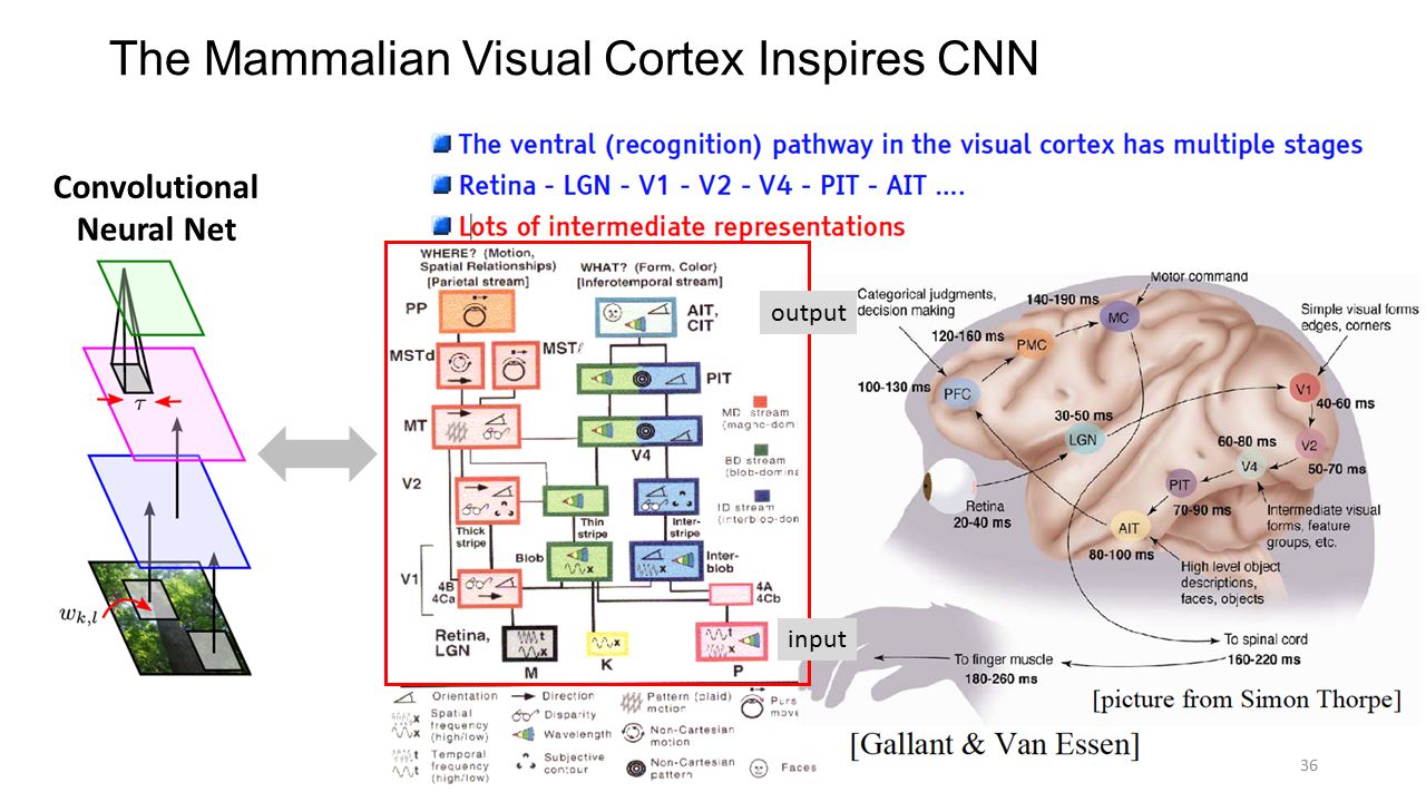
_{^{https://slideplayer.com/slide/10202369/34/images/36/The+Mammalian+Visual+Cortex+Inspires+CNN.jpg}}

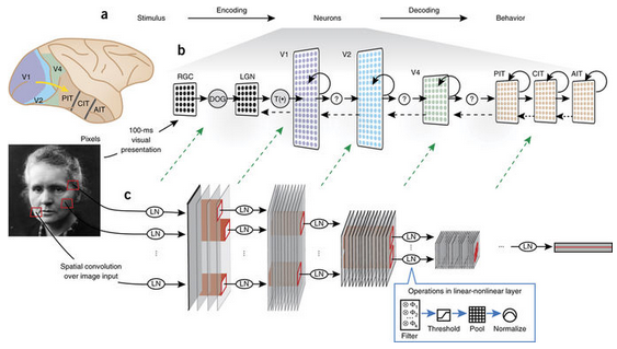
^{Grace Lindsay, https://neurdiness.files.wordpress.com/2018/05/screenshot-from-2018-05-17-20-24-45.png}

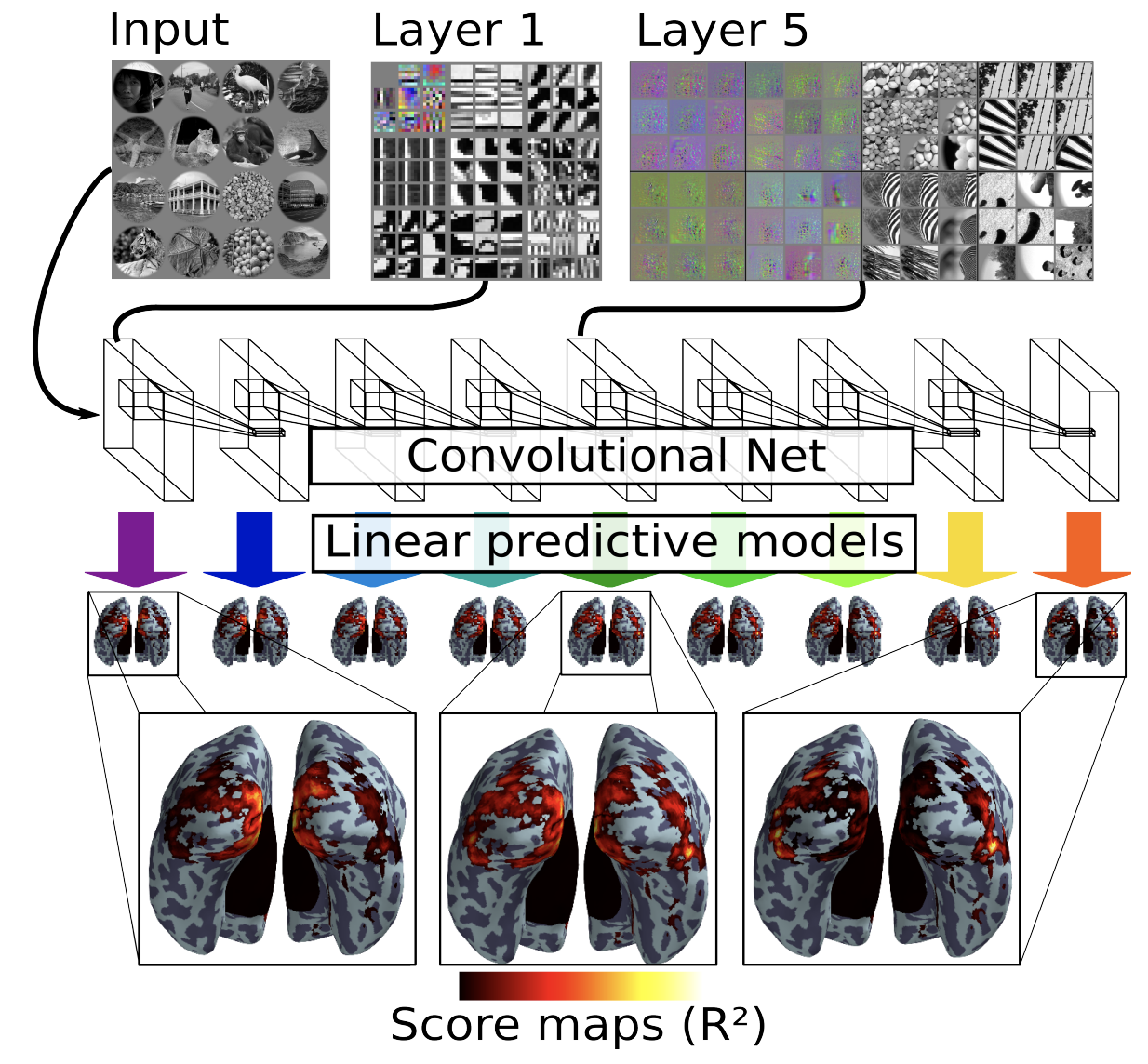
^{Eickenberg et al. 2016, https://hal.inria.fr/hal-01389809/document}

^{Kell et al. 2018, https://doi.org/10.1016/j.neuron.2018.03.044}

The question is still: how do ANNs do that?

From biological to artificial neural neurons and networks

• decades ago researchers started to create artificial neurons to tackle tasks “conventional algorithms” couldn’t handle

• inspired by the learning and performance of biological neurons and networks

• mimic defining aspects of biological neurons and networks

• examples are: integrate and fire neurons, rectified linear rate neuron, perceptrons, multilayer perceptrons, convolutional neural networks, recurrent neural networks, autoencoders, generative adversarial networks

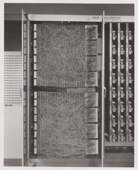
_{^{https://upload.wikimedia.org/wikipedia/en/5/52/Mark_I_perceptron.jpeg}}

• using biological neurons and networks as the basis for artificial neurons and networks might therefore also help to learn invariant representations that capture latent variables

• deep learning = representation learning

• our minds (most likely) contains (invariant) representations about the world that allow us to interact with it

  • task optimization

  • generalizability

Back to biology…

• neurons receive one or more inputs

  • excitatory postsynaptic potentials

  • inhibitory postsynaptic potentials

• inputs are summed up to produce an output

  • an activation

• inputs are separably weighted and sum passed through a non-linear function

  • activation or transfer function

_{^{https://upload.wikimedia.org/wikipedia/commons/thumb/a/ac/Neuron3.svg/2560px-Neuron3.svg.png}}

• these processes can be translated into mathematical problems including the input X, its weights W and the activation function f

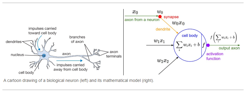
_{^{https://miro.medium.com/max/1400/1*BMSfafFNEpqGFCNU4smPkg.png}}

• the thing about activation functions…

  • they define the resulting type of an artificial neuron

  • thus they also define its capabilities

  • require non-linearity

    • because otherwise only linear functions and decision probabilities

• the thing about activation functions…

\[\begin{split}\begin{array}{l} \text { Non-linear transfer functions}\\ \begin{array}{llc} \hline \text { Name } & \text { Formula } & \text { Year } \\ \hline \text { none } & \mathrm{y}=\mathrm{x} & - \\ \text { sigmoid } & \mathrm{y}=\frac{1}{1+e^{-x}} & 1986 \\ \tanh & \mathrm{y}=\frac{e^{2 x}-1}{e^{2 x}+1} & 1986 \\ \text { ReLU } & \mathrm{y}=\max (\mathrm{x}, 0) & 2010 \\ \text { (centered) SoftPlus } & \mathrm{y}=\ln \left(e^{x}+1\right)-\ln 2 & 2011 \\ \text { LReLU } & \mathrm{y}=\max (\mathrm{x}, \alpha \mathrm{x}), \alpha \approx 0.01 & 2011 \\ \text { maxout } & \mathrm{y}=\max \left(W_{1} \mathrm{x}+b_{1}, W_{2} \mathrm{x}+b_{2}\right) & 2013 \\ \text { APL } & \mathrm{y}=\max (\mathrm{x}, 0)+\sum_{s=1}^{S} a_{i}^{s} \max \left(0,-x+b_{i}^{s}\right) & 2014 \\ \text { VLReLU } & \mathrm{y}=\max (\mathrm{x}, \alpha \mathrm{x}), \alpha \in 0.1,0.5 & 2014 \\ \text { RReLU } & \mathrm{y}=\max (\mathrm{x}, \alpha \mathrm{x}), \alpha=\operatorname{random}(0.1,0.5) & 2015 \\ \text { PReLU } & \mathrm{y}=\max (\mathrm{x}, \alpha \mathrm{x}), \alpha \text { is learnable } & 2015 \\ \text { ELU } & \mathrm{y}=\mathrm{x}, \text { if } \mathrm{x} \geq 0, \text { else } \alpha\left(e^{x}-1\right) & 2015 \\ \hline \end{array} \end{array}\end{split}\]

from IPython.display import IFrame

IFrame(src='https://polarisation.github.io/tfjs-activation-functions/', width=700, height=400)

• historically either sigmoid or tanh utilized

• even though they are non-linear functions their properties make them insufficient for most problems, especially sigmoid

  • rather simple polynomials

  • mainly work for binary problems

  • computationally expensive

  • they saturate causing the neuron and thus network to “die”, i.e. stop learning

• modern ANN frequently use continuous activation functions like Rectified Linear Unit

  • doesn’t saturate

  • faster training and convergence

  • introduce network sparsity

Still, the question is: how does this help us?

Let’s imagine the following situation:

• we could try to iterate over all possible transformations/functions necessary to enable and/or optimize the output

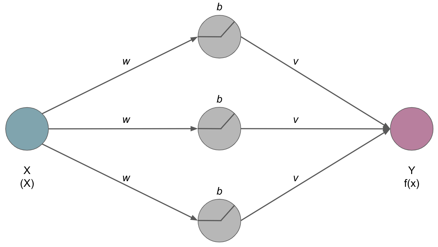
However, we could also introduce a hidden layer that learns or more precisely approximates what those transformations/functions are on its own:

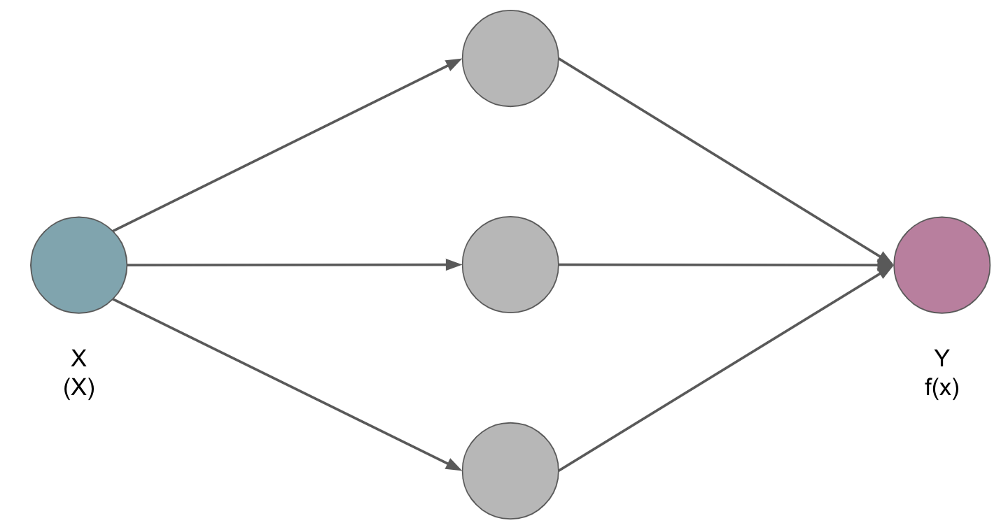
The idea: there is a neural network so that for every possible input X, the outcome is f(X).

Importantly, the hidden layer consists of artificial neurons that perceive weighted inputs w and perform non-linear (non-saturating) activation functions v which output will be used for the task at hand

It gets even better: this holds true even if there are multiple inputs and outputs:

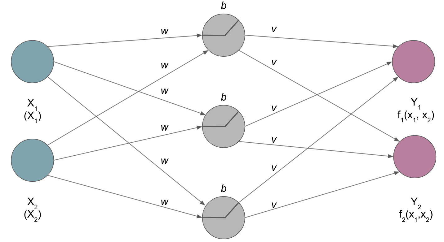
• this is referred to as universality and finally brings us to one core aspect of deep learning

Universal function approximation theorem

• artificial neural networks are considered universal function approximators

  • the possibility of approximating a(ny) function to some accuracy with
    (a set of) artificial neurons in hidden layer

  • instead of providing a predetermined set of transformations or functions, the ANN learns/approximates them by itself

• two problems:

  • the theorem doesn’t tell us how many artificial neurons we need

  • either arbitrary number of artificial neurons (“arbitrary width” case) or arbitrary number of hidden layers, each containing a limited number of artificial neurons (“arbitrary depth” case)

• going back to “shallow learning”: we provide pre-extracted/pre-computed features of our data X and maybe apply further preprocessing before letting our model M learns the mapping to our outcome Y via optimization (minimizing the loss function)

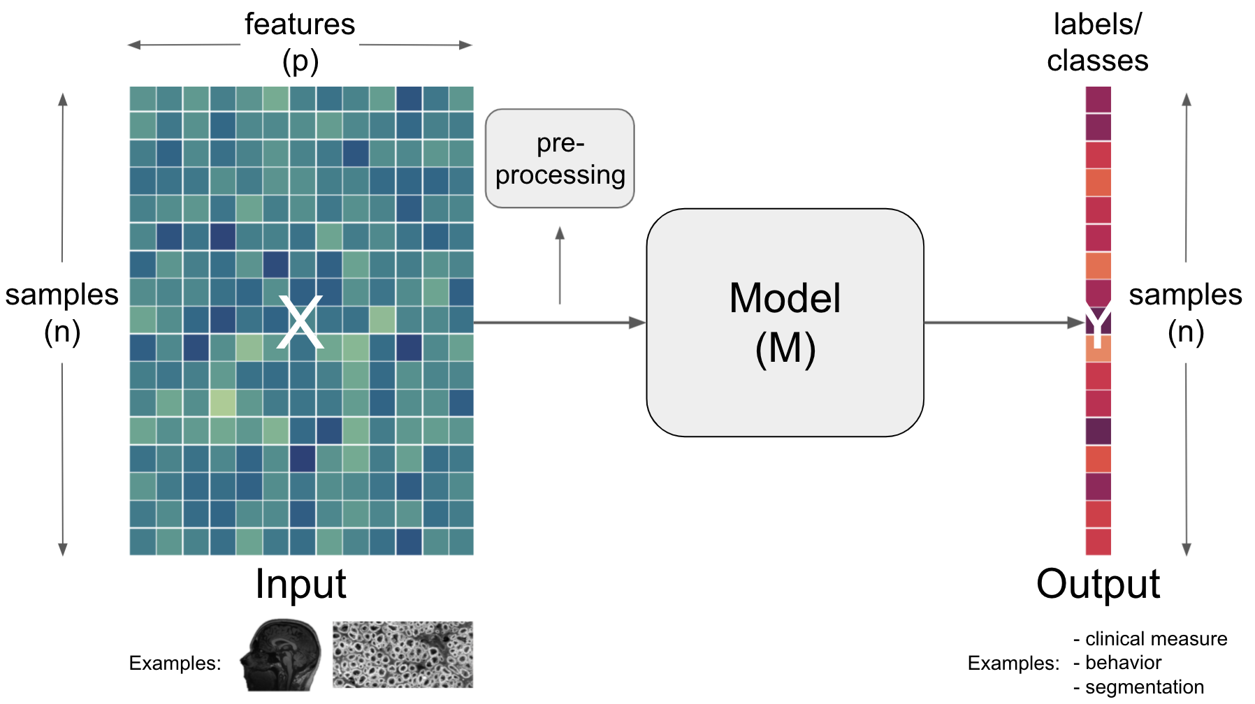
• as it’s very cumbersome to nearly impossible to iterate over all possible features, functions and parameters what deep learning does instead is to learn features by itself, namely those that are most useful for the objective function, e.g. minimize loss for a given task as defined by optimization

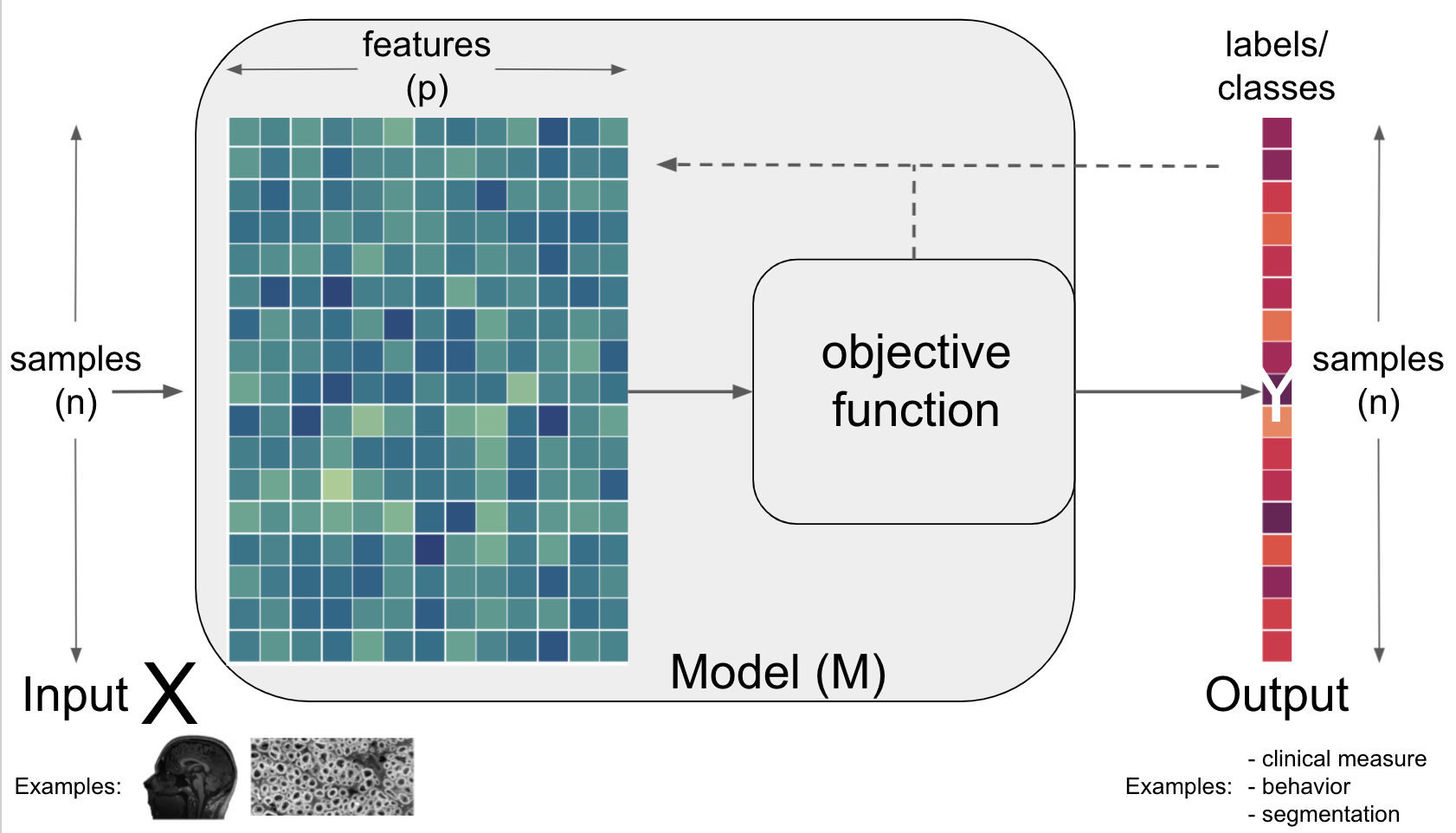
To bring the things we talked about so far together, we will focus on ANN components and how learning takes place next…but at first, let’s take a breather.

_{^{https://media4.giphy.com/media/1LmBFphV4XNSw/giphy.gif?cid=ecf05e47og07li3vrdt89rgz8uux1qjicb3ykg2z5qdgigu7&rid=giphy.gif&ct=g}}

Components of ANNs

• now that we’ve spent quite some time on the neurobiological informed underpinnings it’s time to put the respective pieces together and see how they are actually employed within ANNs

• for this we will talk about two aspects:

  • building blocks of ANNs

  • learning in ANNs

Building blocks of ANNs

• we’ve actually already seen quite a few important building blocks before but didn’t defined them appropriately

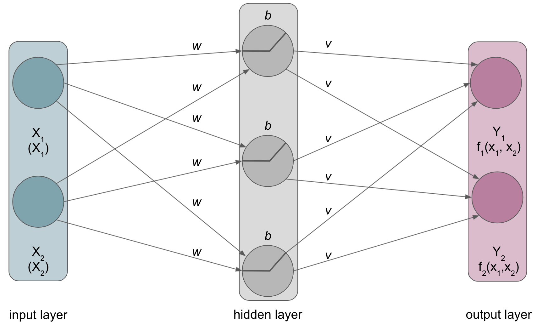
Term	Definition
Layer	Structure or network topology in the architecture of the model that consists of nodes and is connected to other layers, receiving and passing information.
Input layer	The layer that receives the external input data.
Hidden layer(s)	The layer(s) between input and output layer which performs transformations via non-linear activation functions .
Output layer	The layer that produces the final output/task.

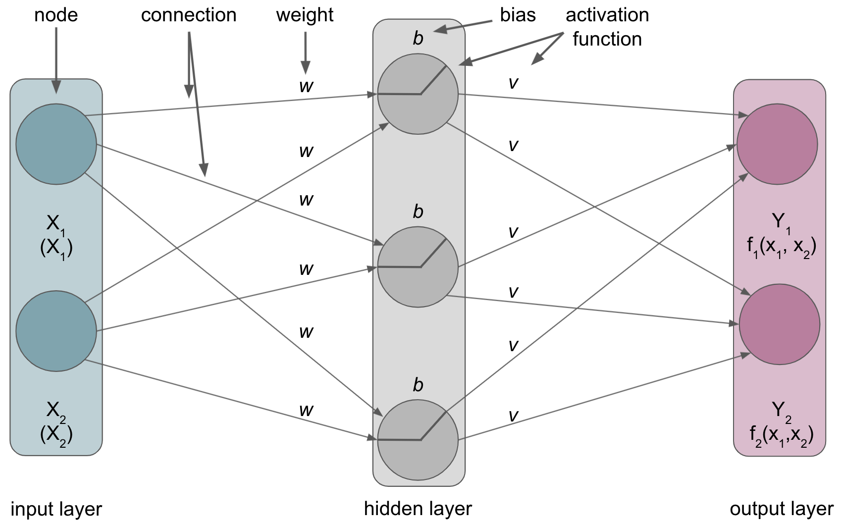
Term	Definition
Node	Artificial neurons.
Connection	Connection between nodes, providing output of one node/neuron as input to the next node/neuron.
Weight	The relative importance of the connection.
Bias	The bias term that can be added to the propagation function, i.e. input to a neuron computed from the outputs of its predecessor neurons and their connections as a weighted sum.

• ANNs can be described based on their amount of hidden layers (depth, width)

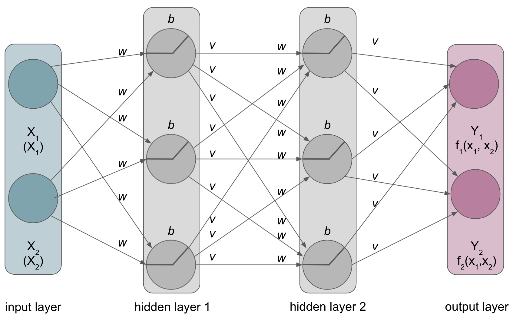
• having talked about overt building blocks of ANNs we need to talk about building blocks that are rather covert, that is the aspects that define how ANNs learn…

Learning in ANNs

• let’s go back a few hours and talk about model fitting again

• when talking about model fitting, we need to talk about three central aspects:

  • the model

  • the loss function

  • the optimization

Term	Definition
Model	A set of parameters that makes a prediction based on a given input. The parameter values are fitted to available data.
Loss function	A function that evaluates how well your algorithm models your dataset
Optimization	A function that tries to minimize the loss via updating model parameters.

An example: linear regression

• Model: $\(y=\beta_{0}+\beta_{1} x_{1}^{2}+\beta_{2} x_{2}^{2}\)$

• Loss function: $\( M S E=\frac{1}{n} \sum_{i=1}^{n}\left(y_{i}-\hat{y}_{i}\right)^{2}\)$

• optimization: Gradient descent

• Gradient descent with a single input variable and n samples

  • Start with random weights (β0 and β1) $\(\hat{y}_{i}=\beta_{0}+\beta_{1} X_{i}\)$

  • Compute loss (i.e. MSE) $\(M S E=\frac{1}{n} \sum_{i=1}^{n}\left(y_{i}-\hat{y}_{i}\right)^{2}\)$

  • Update weights based on the gradient

_{^{https://cdn.hackernoon.com/hn-images/0*D7zG46WrdKx54pbU.gif}}

• Gradient descent for complex models with non-convex loss functions

  • Start with random weights (β0 and β1) $\(\hat{y}_{i}=\beta_{0}+\beta_{1} X_{i}\)$

  • Compute loss (i.e. MSE) $\(M S E=\frac{1}{n} \sum_{i=1}^{n}\left(y_{i}-\hat{y}_{i}\right)^{2}\)$

  • Update weights based on the gradient

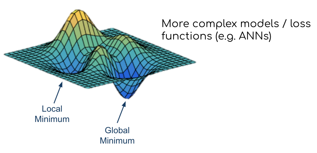
• to sufficiently talk about learning in ANNs we need to add a few things, however we heard some of them already

  • metric

  • activation function

  • weights

  • batch size

  • gradient descent

  • backpropagation

  • epoch

  • regularization

• as you can see, this is going to be something else but we will be trying to bring everything together for a holistic overview

Remember how we talked about the different learning problems? As noted before, the initial idea of deep learning/AI was rather centered around unsupervised or self-supervised learning problems. However, based on the limited success of corresponding models and the outstanding performance of supervised models, the latter where way more heavily applied and focused on. Unfortunately, this workshop won’t be an exception to that. First of all given time and computational resources and second because we though it might be easier to go through the above mentioned things based on a supervised learning problem. If you disagree, please let us know! We will however go through some other learning problems later, e.g. when checking out different architectures and (hopefully) during the practical session where we’ll evaluate what’s possible with your datasets!

For now, we will keep it rather simple and bring back our cats, assuming we want to train the example ANN of the building blocks part to recognize and distinguish them from other animals. To keep it neuroscience related in our minds we could also assume it’s about different brain tissue classes, cell types, etc. .

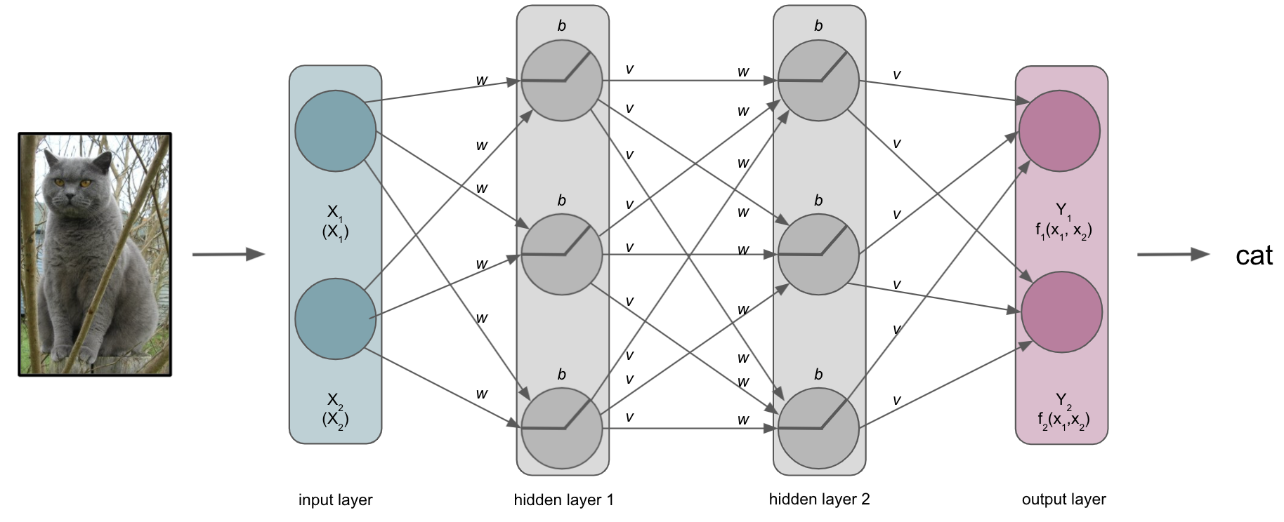
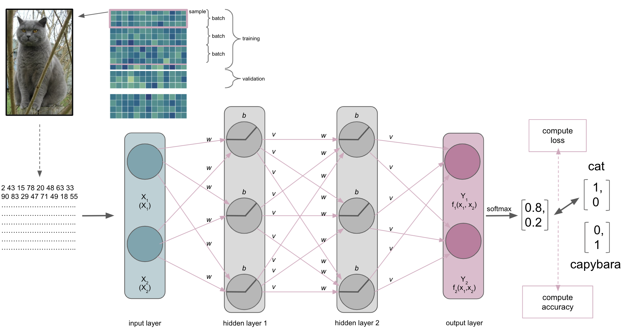
Our ANN receives an input, here an image, and should conduct a certain task, here recognizing/predicting the animal that is shown.

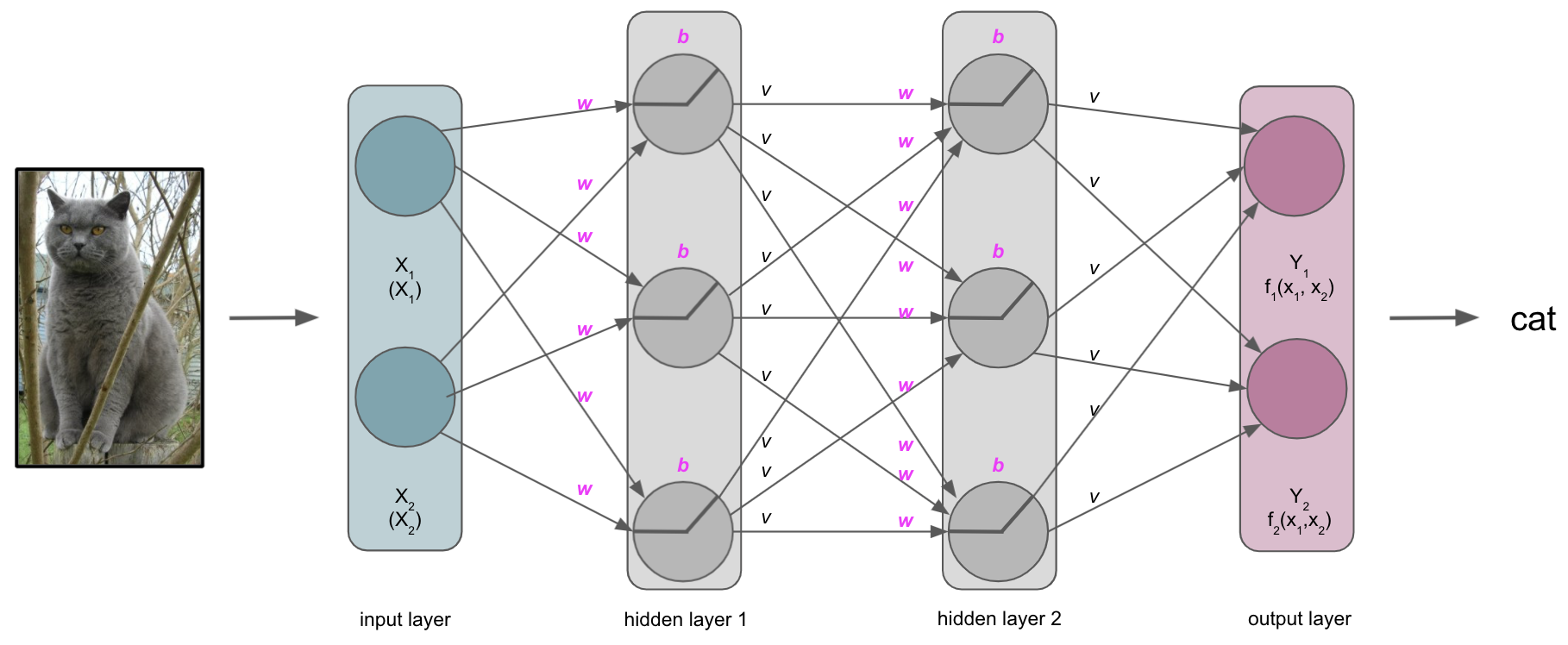
Initialization of weights & biases

Upon building our network we also need to initialize the weights and biases. Both are important hyper-parameters for our ANN and the way it learns as they can help preventing activation function outputs from exploding or vanishing when moving through the ANN. This relates directly to the optimization as the loss gradient might become too large or too small, prolonging the time the network needs to converge or even prevents it completely. Importantly, certain initializers work better with certain activation functions. For example: tanh likes Glorot/Xavier initialization while ReLu likes He initialization.

from IPython.display import IFrame

IFrame(src='https://www.deeplearning.ai/ai-notes/initialization/', width=1000, height=400)

The input layer & the semantic gap

One thing we need to talk about is what the ANN, or more precisely the input layer, actually receives… The same thing, that is the picture of the cat, is very different for us than for a computer. This is referred to as the semantic gap: the transformation of human actions & percepts into computational representations. This picture of a majestic cat is nothing but a huge array for the computer and also what will be submitted to the input layer of the ANN (note: this also holds true for basically any other type of data).

It thus important to synchronize the dimensions of the input and the input shape/size of the input layer. This will also define the datasets you can train and test an ANN on. For example, if you want to work with MRI volumes that have the dimensions [40, 56, 50] or microscopy images with [300, 200, 3], your input layer should have the same input shape/size. The same holds true for all other data you want to train and test your ANN on. Otherwise you would need to redefine the input layer.

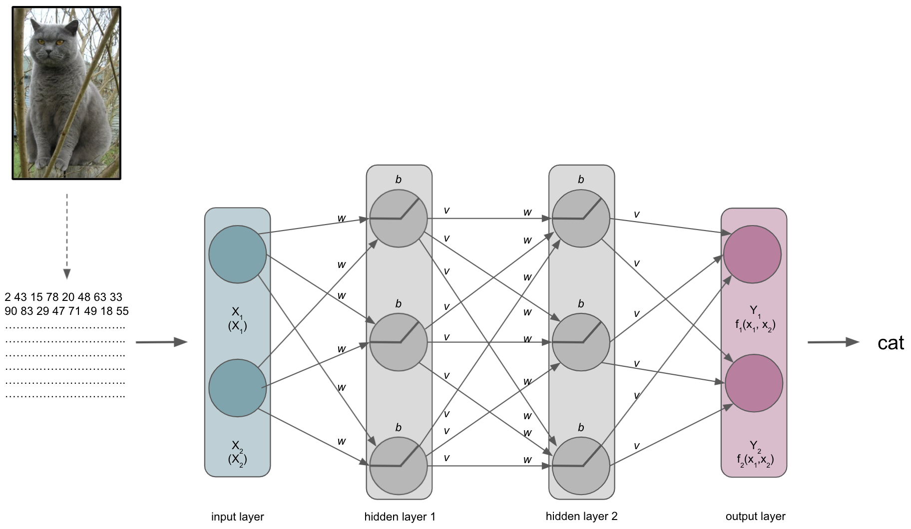
Please note that our example is therefore drastically over-simplified as we would need waaaay more nodes or could just input 2 values.

A journey through the ANN

The input is then processed by the layers, their nodes and respective activation functions, being passed through the ANN. Each layer and node will compute a certain transformation of the input it receives from the previous layer based on its activation function and weights/biases.

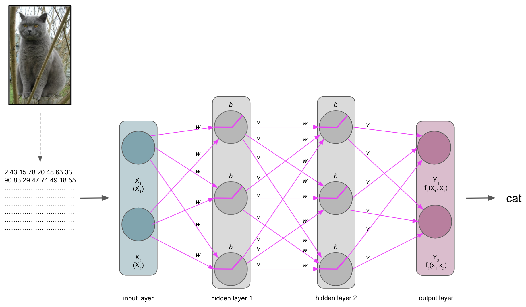
The output layer

After a while, we will reach the end of our ANN, the output layer. As the last part of our ANN, it will produce the results we’re interested in. Its number of nodes and activation function will depend on the learning problem at hand. For a binary classification task it will have 2 nodes corresponding to the both classes and might use sigmoid or softmax activation function. For multiclass classification tasks it will have as many nodes as there are classes and utilize the softmax activation function. Both sigmoid and softmax are related to logistic regression, with the latter being a generalized form of it. Why does this matter? Our output layer will produce real-valued scores for each of the classes that are however not scaled and straightforward to interpret. Using for example the softmax function we can transform these values into scaled probability distributions between 0 and 1 which values add up to 1 and can be submitted to other analysis pipelines or directly evaluated.

Lets assume our ANN is trained to recognize and distinguish cats and capybaras, meaning we have a binary classification task. Defining cats as class 1 and capybaras as class 2 (not my opinion, just an example), the corresponding vectors we would like to obtain from the output layer would be [1,0] and [0,1] respectively. However, what we would get from the output layer in absence of e.g. softmax, would rather look like [1.6, 0.2] and [0.4, 1.2]. This is identical to what the penultimate layer would provide as input the output i.e. softmax layer if we had an additional layer just for that and not the respective activation function.

After passing through the softmax layer or our output layer with softmax activation function the real-valued scores [1.6, 0.2] and [0.4, 1.2] would be (for example) [0.802, 0.198] and [0.310, 0.699]. Knowing it’s now a scaled probabilistic distribution that can range between 0 and 1 and sums up to 1, it’s much easier to interpret.

The metric

The index of the vector provided by the softmax output layer with the largest value will be treated as the class predicted by the ANN, which in our example would be “cat”. The ANN will then use the predicted class and compare it to the true class, computing a metric to assess its performance. Remember folks: deep learning is machine learning and computing a metric is no exception to that. Thus, depending on your data and learning problem you can indicate a variety of metrics your ANN should utilize, including accuracy, F1, AUC, etc. . Note: in binary tasks usually only the largest value is treated as a class prediction, this is called Top-1 accuracy. On the contrary, in multiclass tasks with many classes (animals, cell components, disease propagation types, etc.) quite often the largest 5 values are treated as class predictions and utilized within the metric, which is called Top-5 accuracy.

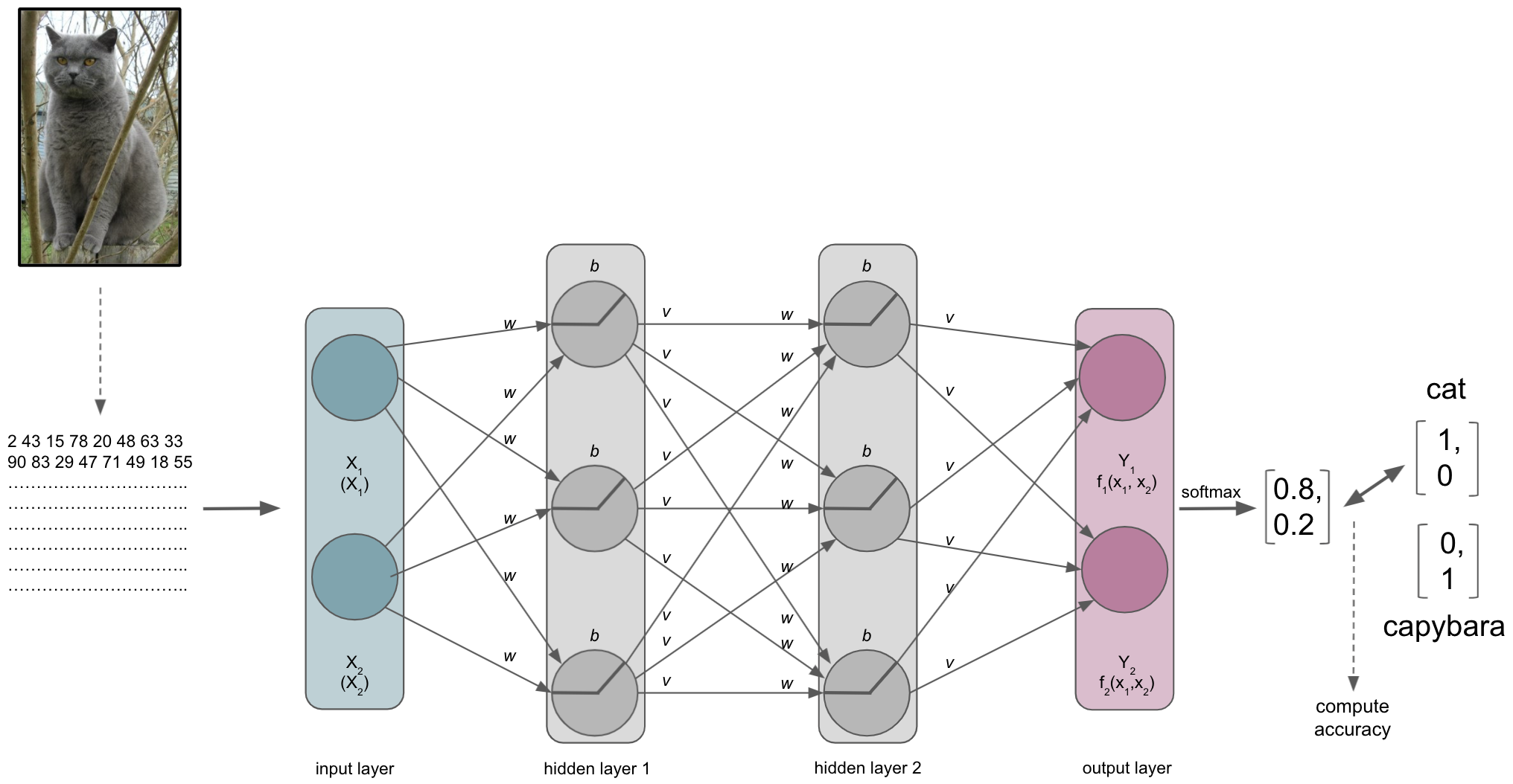
The loss function

Besides the metric, our ANN will also a compute a loss function that will quantify how far the probabilities, computed by the softmax function of the output layer, are away from the true values we want to achieve, i.e. the classes. As mentioned in the introduction and comparable to the metric, the choice of loss function depends on the data you have and the learning problem you want to solve. If you want to predict numerical values you might want to employ a regression based approach and use MSE as the loss function. If you want to predict classes you might to employ a classification based approach and use a form of cross-entropy as the loss function.

A cool thing about softmax with regard to the loss function: it is a continuously differentiable function and thus the derivative of the loss function can be computed for every weight and every input in the training set. Based on that the weights of the ANN can be adapted to reduce the loss function, making the predicted values provided by the output layer closer to the true values (i.e. classes) and therefore improving the metric and performance of the ANN. This reducing of the error (assessed through the loss function) is called the objective function of an ANN, while the adaptation of weights to improve the performance of an ANN is the learning process. But how does this work now? We know it has something to do with optimization…Let’s have a look when and how this factors in.

Batch size

As with other machine learning approaches, we will ideally have a training, validation and test set. One hyperparameter that is involved in this process and also can define our entire learning process is batch size. It defines the number of samples in the training set our ANN processes before optimization is used to update the weights based on the result of the loss function. For example, if our training set has 100 samples and we set a batch size of 5, we would divide the training set into 20 batches of 5 samples each. In turn this would mean that our ANN goes through 5 samples before using optimization to update the weights and thus our ANN would update its weights 20 times during training.

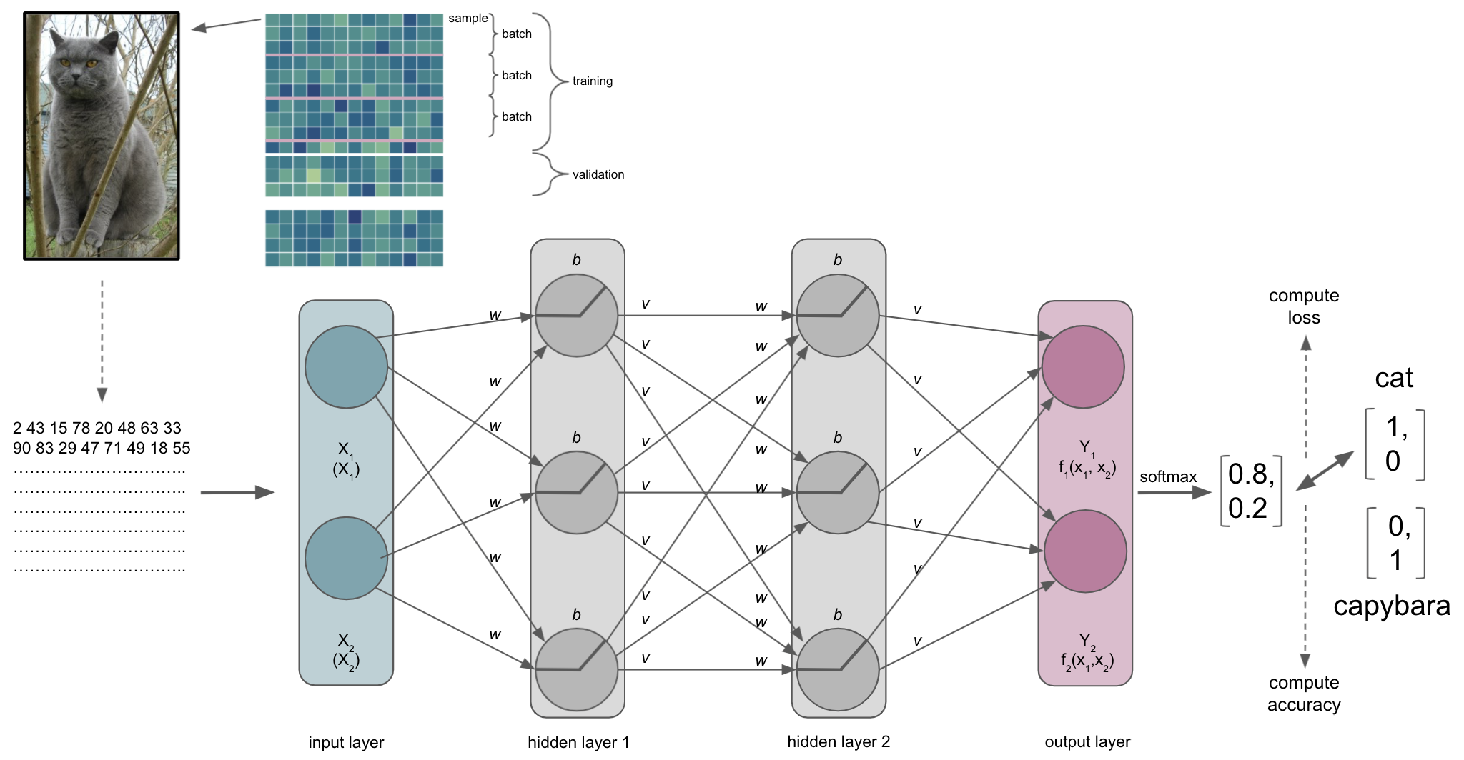
The optimization

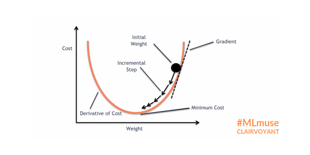
Once a batch has been processed by the ANN the optimization algorithm will get to work. As mentioned before, most machine learning problems utilize gradient descent as the optimization algorithm. As mentioned during the introduction and a few slides above, we have an objective function we want to optimize, for example minimizing the error computed by our cross-entropy loss function. So what happens is the following. At first, an entire batch is processed by the ANN and accuracy as well as loss are computed.

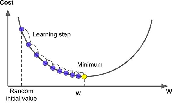
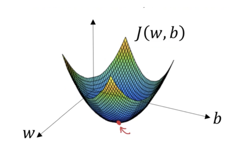
Subsequently, the error computed via the loss function will be minimized through gradient descent. Let’s imagine the following: we span a valley-looking like gradient that is defined by our weights and biases on the horizontal or x and y axes and the loss function on the vertical or z axis. This is where our weight and bias initializers come back: we initialized weights and biases at a certain point on the gradient, usually on the top or quite high. Now our optimization algorithm takes one step after another (after each batch) in the steepest downwards direction along the gradient via finding weights and biases that reduce the loss until it reaches the point where the error computed by the loss function is as small as possible. It is descending through the gradient. When it reaches this point, i.e. the error can’t be reduced anymore and remains stable, it has converged.

_{^{https://miro.medium.com/max/1024/1*G1v2WBigWmNzoMuKOYQV_g.png}}

Let’s have a look at a few more graphics:

_{^{https://miro.medium.com/max/600/1*iNPHcCxIvcm7RwkRaMTx1g.jpeg}}

_{^{https://cdn.builtin.com/sites/www.builtin.com/files/styles/ckeditor_optimize/public/inline-images/national/gradient-descent-convex-function.png}}

_{^{https://blog.paperspace.com/content/images/2018/05/fastlr.png}}

Check this cool project, called loss landscape by Javier Ideami:

from IPython.display import IFrame

IFrame(src='https://losslandscape.com/explorer', width=700, height=400)

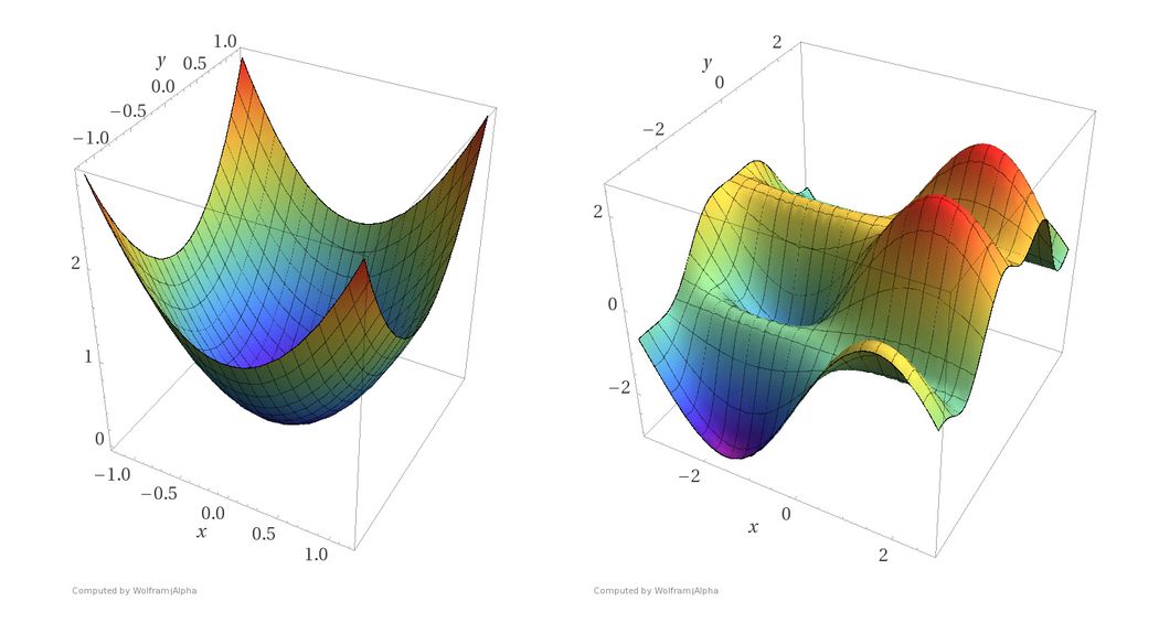
What this shows nicely is one aspect we briefly discussed during the introduction: ANNs are complex models and result in non-convex loss functions, i.e. gradients with a global minimum/maximum and various local ones.

_{^{https://blog.paperspace.com/content/images/size/w1050/2018/05/convex_cost_function.jpg}}

So chances are, our gradient descent will get stuck in a local minimum and won’t find the global minimum. At least that’s what people thought in the beginning….

As it turned out, gradient desecent rather gets stuck in what is called saddle points

_{^{https://www.offconvex.org/assets/saddle/minmaxsaddle.png}}

The thing is: in order to find a local or global minimum all the dimensions, i.e. parameters(weights/biases) must agree to this point. However, what happens mostly in complex models with millions of parameters is that only a subset of dimensions agree which creates saddle points.

There are however newer algorithms that help gradient descent getting out of saddle points, for example adam.

This brings us to some other important aspects of gradient descent:

• types

• learning rate

In general, gradient descent is divided into three types:

• batch gradient descent

• stochastic gradient descent

• mini batch gradient descent

In batch gradient descent the error is computed for each sample of the training set, but model will only be updated once the entire training set was processed.

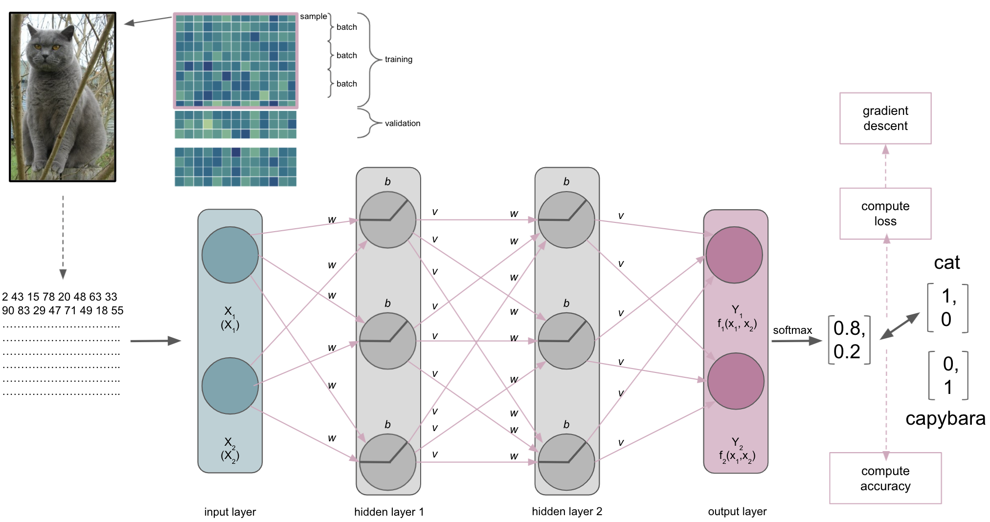
In stochastic gradient descent the error is computed for each sampleof the training set and model immediately updated.

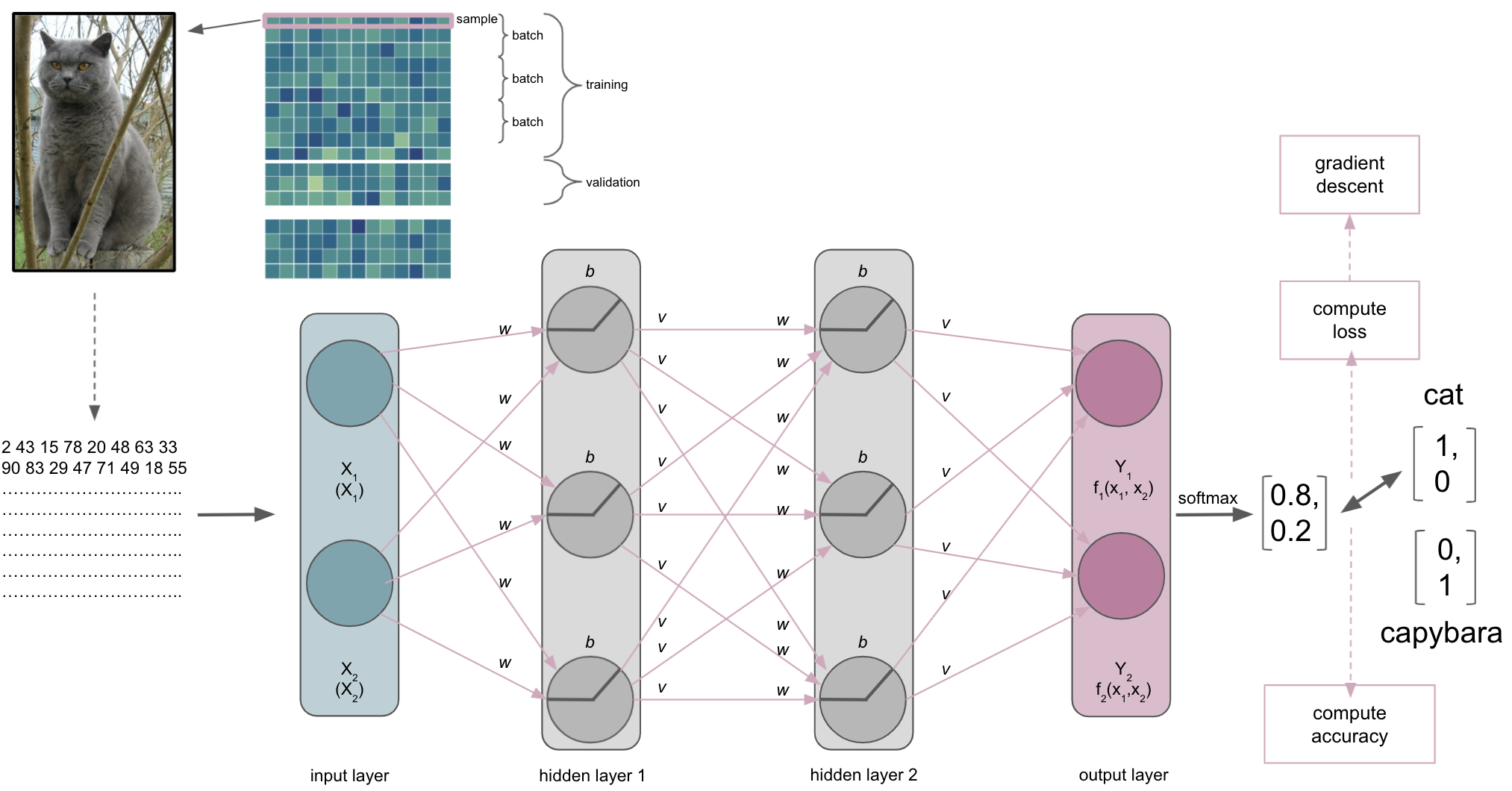
In mini-batch gradient descent the error is computed for a subset of the training set and the model updated after each of those batches. It is commonly used, as it combines the robustness of stochastic gradient descent and the efficiency of batch gradient descent.

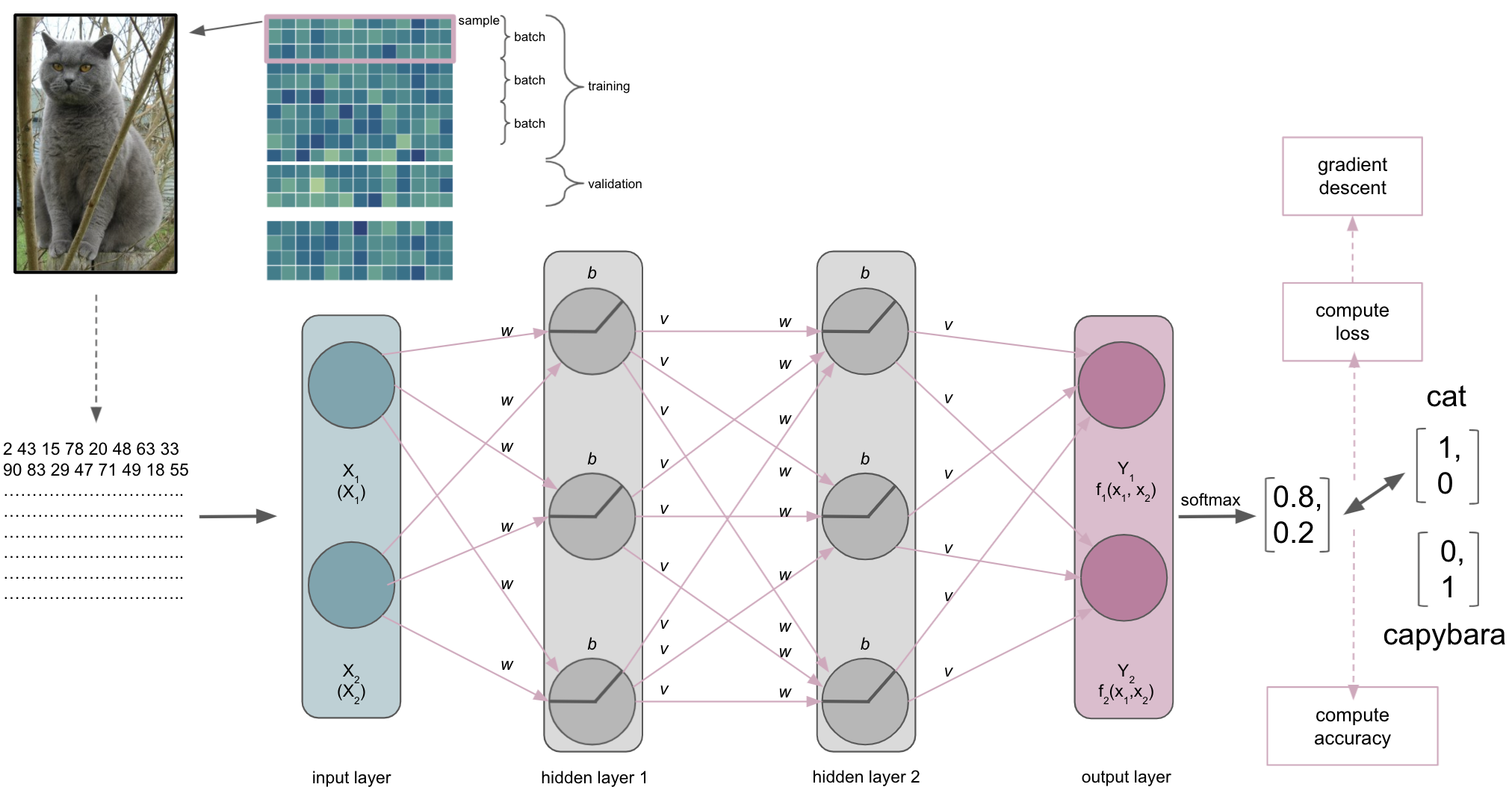
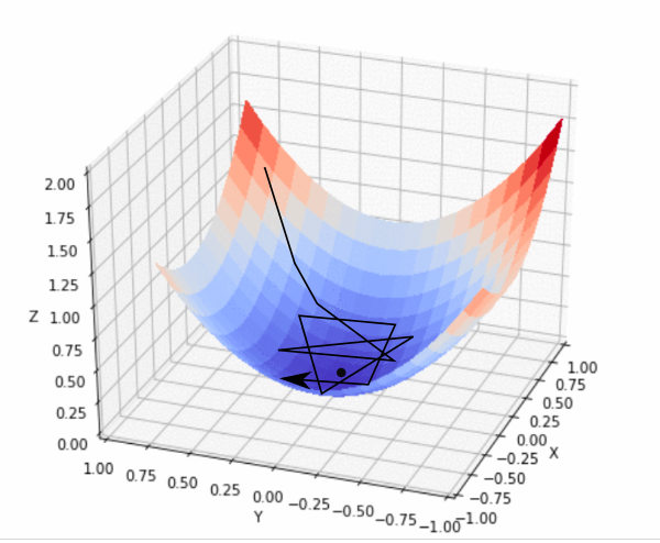
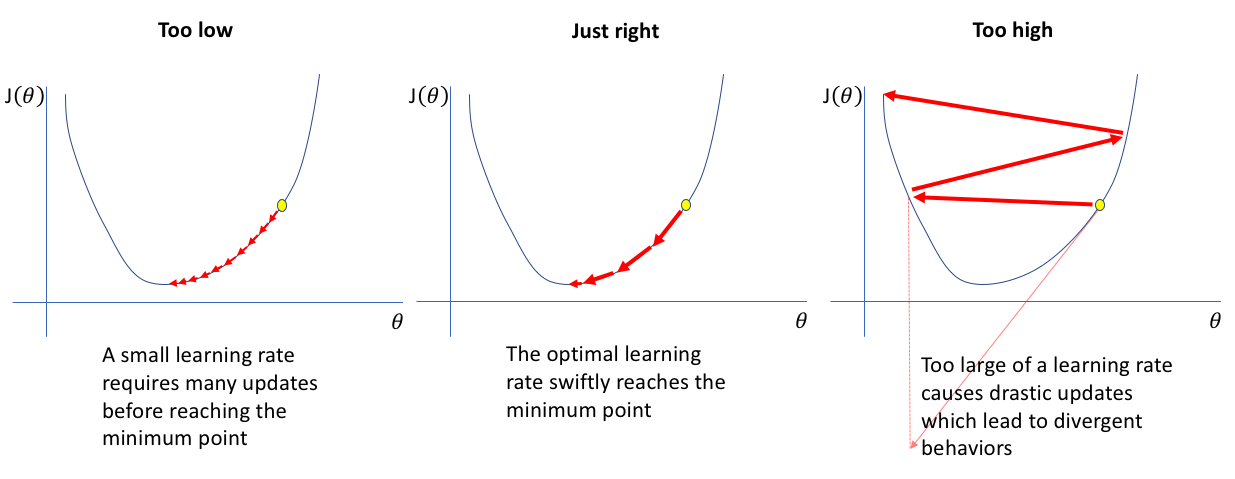
Another important aspect of gradient descent is the learning rate which describes how big the steps are the gradient descent takes towards the minimum. If the learning rate is too high, i.e. the steps too big it might bounce back and forth without being able to find the minimum. If the learning rate is too small, i.e. the steps too small it might take a very long time to find the minimum.

_{^{https://www.jeremyjordan.me/content/images/2018/02/Screen-Shot-2018-02-24-at-11.47.09-AM.png}}

Now that we spend some time on gradient descent as an optimization algorithm, there’s still the question how the parameters, weights and biases, of our ANN are actually updated.

Backpropagation

Actually, gradient descent is part of something bigger called backpropagation. Once we did a forward pass through the ANN, i.e. data goes from input to output layer, the ANN will use backpropagation to update the model parameters. It does so by utilizing gradient descent and the chain rule to propagate the error backwards. Simply put: starting at the output layer gradient descent is applied to update its parameters, i.e. weights and biases, the error is re-computed through the loss function and propagated backwards to the previous layer, where parameters will be updated, the error re-computed through the loss function and so forth. As parameters interact with each other, the application of the chain rule is important as it can decompose the composition of two differentiable functions into their derivatives.

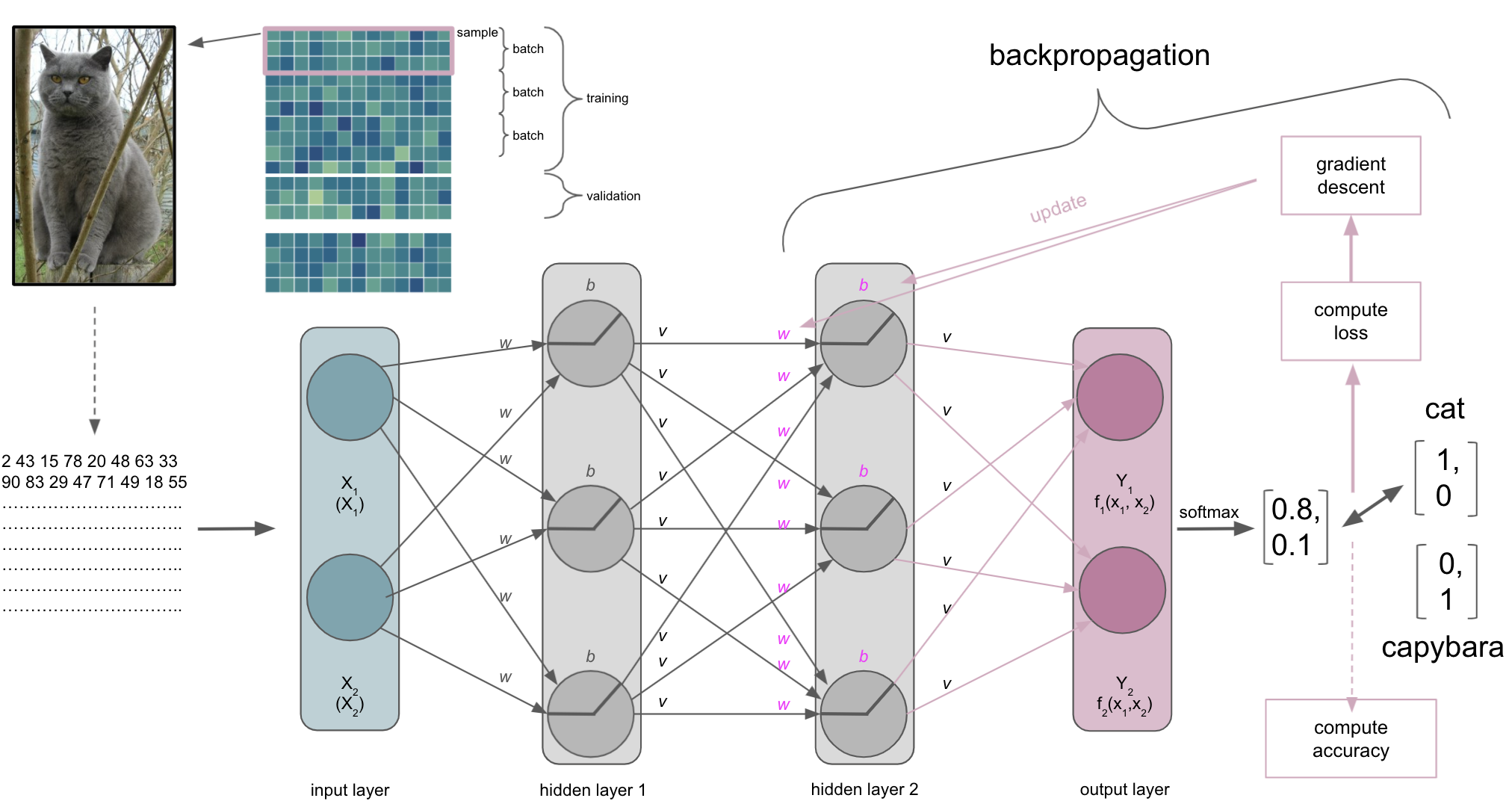
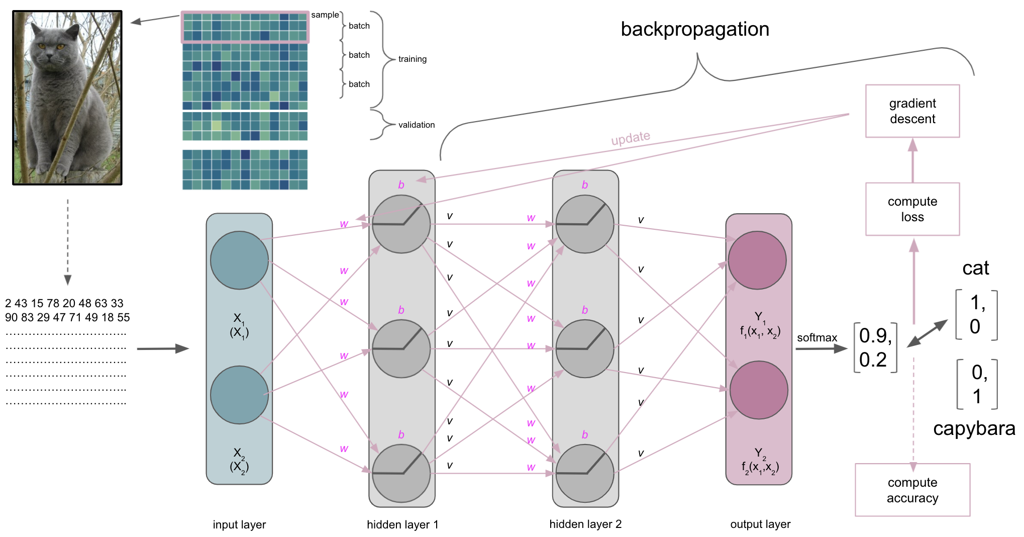
We almost have everything together…almost. One thing we still haven’t talked about is how long this entire composition of processes will run.

The number of epochs

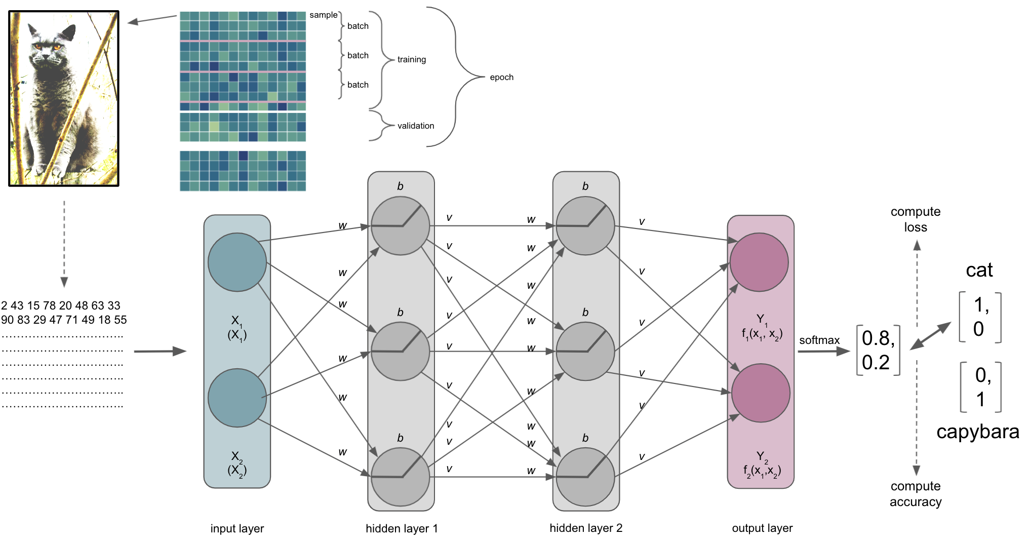
The duration of the ANN training is usually determined by the interplay between batch sizes and another hyperparameter called epochs. Whereas the batch size defines the number of training set samples to process before updating the model parameters, the number of epochs specifies how often the ANN should process the entire training set. Thus, once all batches have been processed, one epoch is over. The number of epochs is something you set when start the training, just like the batch size. Both are therefore parameters for the training and not parameters that are learned by the training. For example, if you have 100 samples, a batch size of 10 and set the number of epochs to 500 your ANN will go through the entire training set 500 times, that is 5000 batches and thus 5000 updates to your model. While this sounds already like a lot, these numbers are more than small compared to that what “real-life” ANNs go through. There, these numbers are in the millions and beyond.

Please note: this is of course only the theoretical duration in terms of iterations and not the actual duration it takes to train your ANN. This is quite often hard to predict (hehe, got it?) as it depends on the computational setup you’re working with, the data and obviously the model and its hyperparameters.

Stop y’all, we forgot something!

_{^{https://c.tenor.com/420FjCVLWbMAAAAM/dog-cachorro.gif}}

The regularitzation

Does this ring a bell? That’s right: it’s still machine learning and thus, as with every model, we need to address overfitting and underfitting, especially with this amount of parameters.

_{^{https://miro.medium.com/max/1396/1*lARssDbZVTvk4S-Dk1g-eA.png}}

_{^{https://miro.medium.com/max/1380/1*rPStEZrcv5rwu4ulACcwYA.png}}

There are actually multiple types of regularization we can apply to help our ANN to generalize better (other than increasing the size of the training set):

• L1/L2 regularization

• dropout

• data augmentation

• early stopping

Using L1/L2 regularization (the most common type of regularization), we add a regularization term (L1 or L2) to our loss function that will decrease the weights assuming that models with smaller weights will lead to less complex models that in turn generalize better.

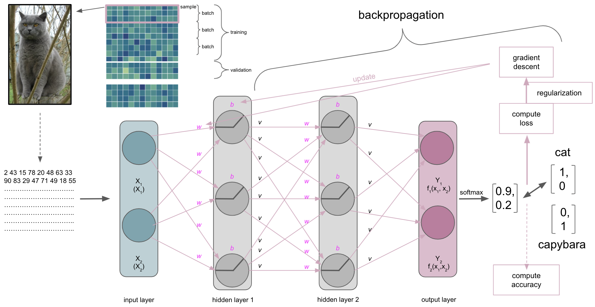
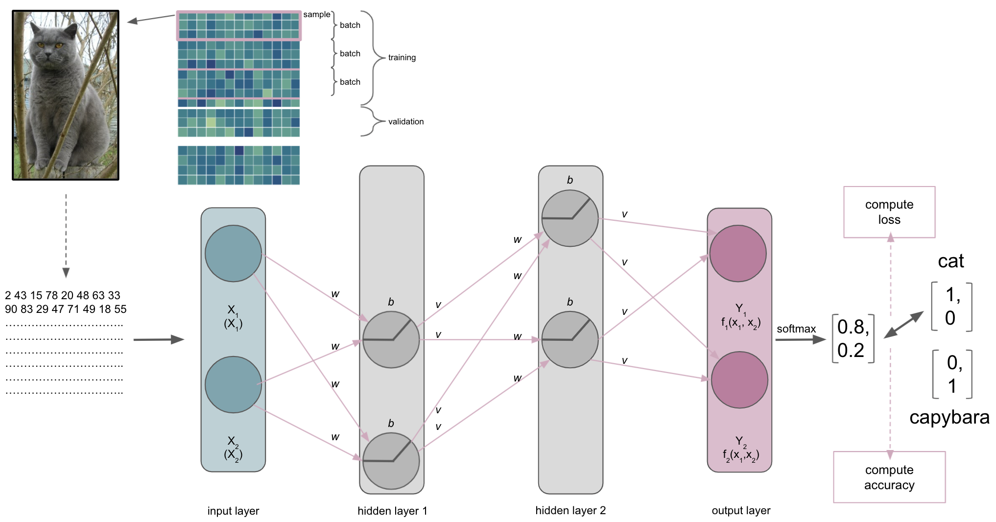
Using dropout, we regularize by randomly and temporally dropping nodes and their corresponding connections, thus efficiently changing the ANN architecture and introducing a certain amount of randomness. (Does this regularization approach remind you of one of the models we saw during the “classic” machine learning part?).

Using data augmentation, we regularize without directly changing parts of the ANN but changing the training set. To be more precise, not really “changing the training set” but adding “changed” versions of the training set samples, i.e. the same samples but in an altered form. For example, if we work with images (MRI volumes, microscopy, etc.) we could shear, shift, scale and rotate the images, as well as adding noise, etc. . (Think about invariant representations again.)

When using early stopping we regularize by stopping the training before the ANN can start to overfit on the training set, for example if the validation error stops decreasing.

_{^{https://miro.medium.com/max/567/1*2BvEinjHM4SXt2ge0MOi4w.png}}

Talking about stopping…this concludes our adventure into learning in ANNs.

_{^{https://c.tenor.com/87__ss7n4fsAAAAC/stop-cut-it-off.gif}}

ANN architectures

• now that we’ve gone through the underlying basics and important building blocks of ANNs, we will check out a few of the most commonly used architectures

• in general we can group ANNs based on their architecture, that is how their building blocks are defined and integrated

• possible architectures include (only a very tiny subset listed):

  • feedforward (information moves in a forward fashion through the ANN, without cycles and/or loops)

    • Multilayer perceptrons

    • Convolutional neural networks

    • autoencoders

  • recurrent (information moves in a forward and a backward fashion through the ANN)

    • fully recurrent

    • Long short-term memory

  • radial basis function (networks that use radial basis functions as activation function)

    • General regression network

    • Deep belief networks

• we will spend a closer look at feedforward and recurrent architectures as they will (most likely) be the ones you see frequently utilized within neuroscience

• however, to see how well we explained things to you (and because we’re lazy): we would like to ask y’all to form 5 groups and each group will get 5 min to find something out about 1 ANN architecture

• after that, we will of course also add respective slides to this section!

The moral of the story

We heard, saw and learned that deep learning can be and already is very powerful but …

_{^{https://thinkingmeme.com/wp-content/uploads/2018/07/Top-24-Jeff-Goldblum-memes21.jpg}}

Yes it’s super cool. Yes, it’s basically THE BUZZWORD. However, before applying deep learning you should ask yourself:

• does my task involve a hierarchy?

• what computational and time resources do I have?

• is there enough data?

• are there pre-trained models?

• are there datasets I could pre-train my model on?

(This slide and all that follow stolen from Blake Richards)

Quite often, deep learning won’t be the answer…!

• a highly recommended read:

Schulz et al. 2020

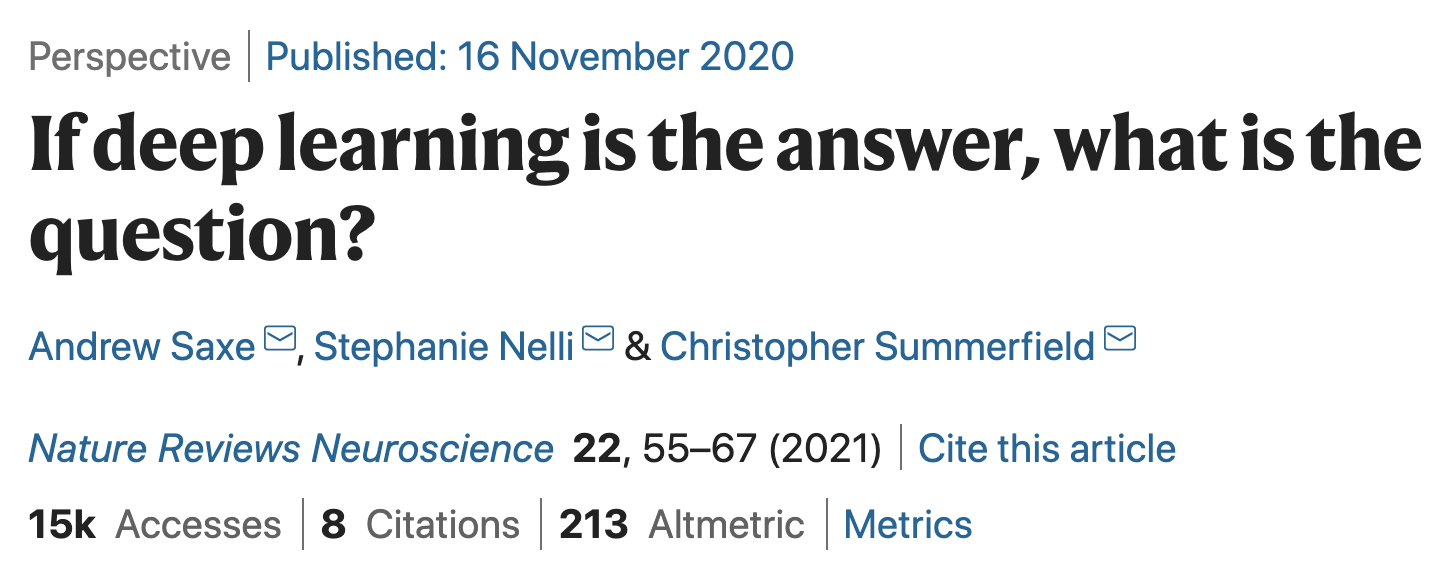
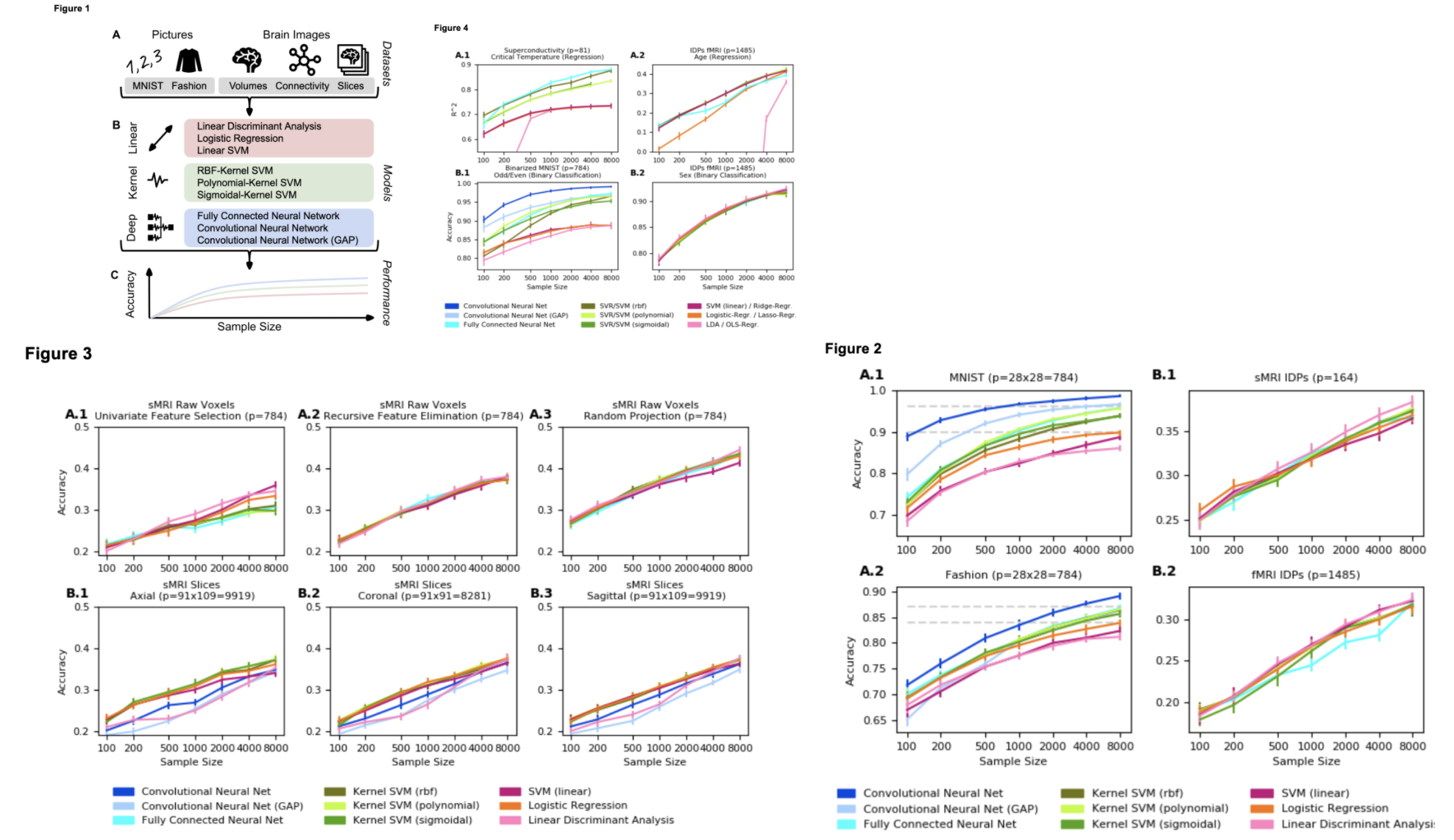
But sometimes it can be…

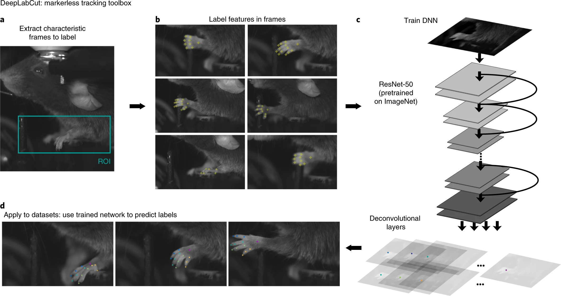
^{DeepLabCut by Mathis et al. 2018}

When to use deep learning:

• it is powerful but intended for the AI set, tasks humans and animals are good at

• it uses an inductive bias of hierarchy, which can be really useful or not at all

• effective when you have a huge model and a huge amount of data

When not to use deep learning:

• no reason to assume the problem contains a hierarchical solution

• limited time & computational resources

• you only have a small amount of data and no related dataset to pre-train

If you don’t really know or can’t really estimate, it’s usually a good idea to stick with other, simpler models as it’s better to stay as general purpose as possible in these cases.

^{https://cdn-images-1.medium.com/fit/t/1600/480/1*rdVotAISnffB6aTzeiETHQ.png}

previous

Deep learning

next

Build and train your neural network