Data analyzes I - basics in data handling
Contents
Data analyzes I - basics in data handling
Peer Herholz (he/him)
Habilitation candidate - Fiebach Lab, Neurocognitive Psychology at Goethe-University Frankfurt
Research affiliate - NeuroDataScience lab at MNI/McGill
Member - BIDS, ReproNim, Brainhack, Neuromod, OHBM SEA-SIG, UNIQUE
![]()
![]() @peerherholz
@peerherholz
Before we get started …
most of what you’ll see within this lecture was prepared by Ross Markello, Michael Notter and Peer Herholz and further adapted for this course by Peer Herholz
based on Tal Yarkoni’s “Introduction to Python” lecture at Neurohackademy 2019
based on 10 minutes to pandas
Objectives 📍
learn basic and efficient usage of python for data analyzes & visualization
working with data:
reading, working, writing
preprocessing, filtering, wrangling
visualizing data:
basic plots
advanced & fancy stuff
Why do data science in Python?
all the general benefits of the
Python language(open source, fast, etc.)Specifically, it’s a widely used/very flexible, high-level, general-purpose, dynamic programming language
the
Python ecosystemcontains tens of thousands of packages, several are very widely used in data science applications:Jupyter: interactive notebooks
Numpy: numerical computing in Python
pandas: data structures for Python
pingouin: statistics in Python
statsmodels: statistics in Python
seaborn: data visualization in Python
plotly: interactive data visualization in Python
Scipy: scientific Python tools
Matplotlib: plotting in Python
scikit-learn: machine learning in Python
even more:
Pythonhas very good (often best-in-class) external packages for almost everythingParticularly important for data science, which draws on a very broad toolkit
Package management is easy (conda, pip)
Examples for further important/central python data science packages :
Web development: flask, Django
Database ORMs: SQLAlchemy, Django ORM (w/ adapters for all major DBs)
Scraping/parsing text/markup: beautifulsoup, scrapy
Natural language processing (NLP): nltk, gensim, textblob
Numerical computation and data analysis: numpy, scipy, pandas, xarray
Machine learning: scikit-learn, Tensorflow, keras
Image processing: pillow, scikit-image, OpenCV
Plotting: matplotlib, seaborn, altair, ggplot, Bokeh
GUI development: pyQT, wxPython
Testing: py.test
Widely-used
Python is the fastest-growing major programming language
Top 3 overall (with JavaScript, Java)

What we will do in this section of the course is a short introduction to Python for data analyses including basic data operations like file reading and wrangling, as well as statistics and data visualization. The goal is to showcase crucial tools/resources and their underlying working principles to allow further more in-depth exploration and direct application.
It is divided into the following chapters:
Getting ready
Basic data operations
Reading data
Exploring data
Data wrangling
Basic data visualization
Underlying principles
“standard” plots
Going further with advanced plots
Statistics in python
Descriptive analyses
Inferential analyses
Interactive data visualization
Here’s what we will focus on in the first block:
Getting ready
Basic data operations
Reading data
Exploring data
Data wrangling
Getting ready
What’s the first thing we have to check/evaluate before we start working with data, no matter if in Python or any other software? That’s right: getting everything ready!
This includes outlining the core workflow and respective steps. Quite often, this notebook and its content included, this entails the following:
What kind of data do I have and where is it?
What is the goal of the data analyses?
How will the respective steps be implemented?
So let’s check these aspects out in slightly more detail.
What kind of data do I have and where is it
The first crucial step is to get a brief idea of the kind of data we have, where it is, etc. to outline the subsequent parts of the workflow (python modules to use, analyses to conduct, etc.). At this point it’s important to note that Python and its modules work tremendously well for basically all kinds of data out there, no matter if behavior, neuroimaging, etc. . To keep things rather simple, we will use a behavioral dataset that contains ratings and demographic information from a group of university students (ah, the classics…).
Knowing that all data files are located in a folder called data_experiment on our desktop, we will use the os module to change our current working directory to our desktop to make things easier:
from os import chdir

chdir('/Users/peerherholz/Desktop/')
Now we can actually already start using Python to explore things further. For example, we can use the glob module to check what files are in this directory and obtain a respective list:
from glob import glob

data_files = glob('data_experiment/*.csv')
As you can see, we provide a path as input to the function and end with an *.csv which means that we would like to gather all files that are in this directory that end with .csv. If you already know more about your data, you could also use other expressions and patterns to restrain the file list to files with a certain name or extension.
So let’s see what we got. Remember, the function should output a list of all files in the specified directory.
data_files
['data_experiment/yagurllea_experiment_2022_Jan_25_1318.csv',
 'data_experiment/pauli4psychopy_experiment_2022_Jan_24_1145.csv',
 'data_experiment/porla_experiment_2022_Jan_24_2154.csv',
 'data_experiment/Sophie Oprée_experiment_2022_Jan_24_1411.csv',
 'data_experiment/participant_123_experiment_2022_Jan_26_1307.csv',
 'data_experiment/funny_ID_experiment_2022_Jan_24_1215.csv',
 'data_experiment/Chiara Ferrandina_experiment_2022_Jan_24_1829.csv',
 'data_experiment/Heidi Klum_experiment_2022_Jan_26_1600.csv',
 'data_experiment/Smitty_Werben_Jagger_Man_Jensen#1_experiment_2022_Jan_26_1158.csv',
 'data_experiment/wile_coyote_2022_Jan_23_1805.csv',
 'data_experiment/bugs_bunny_experiment_2022_Jan_23_1745.csv',
 'data_experiment/Bruce_Wayne_experiment_2022_Jan_23_1605.csv',
 'data_experiment/twentyfour_experiment_2022_Jan_26_1436.csv',
 'data_experiment/Nina _experiment_2022_Jan_24_1212.csv',
 'data_experiment/daffy_duck_experiment_2022_Jan_23_1409.csv']
Coolio, that worked. We get a list indicating all files as items in the form of strings. We also see that we get the relative paths and that our files are in .csv format. Having everything in a list, we can make use of this great python data type and e.g. check how many files we have, as well as if we have a file for every participant (should be 15).
print(len(data_files))

if len(data_files)==15:
    print('The number of data files matches the number of participants.')
elif len(data_files) > 15:
    print('There are %s more data files than participants.' %str(int(len(data_files)-19)))
elif len(data_files) < 15:
    print('There are %s data files missing.' %str(19-len(data_files)))
15
The number of data files matches the number of participants.
We also saw that some files contain a ' ', i.e. space, and knowing that this can cause major problems when coding analyzes, we will use python again to rename them. Specifically, we will use the rename function of the os module. It expects the old file name and the new file name as positional arguments, i.e. os.rename(old_file_name, new_file_name). While renaming, we follow “best practices” and will replace the space with an _. In order to avoid doing this manually for all files, we will just use a combination of a for loop and an if statement:
from os import rename

for file in data_files:
    if ' ' in file:
        rename(file, file.replace(' ', "_"))
Exercise 1
Can you describe what behavior the above lines of code implement?
See how cool and easy the python basics we explored in the introduction can be applied “in the wild”? That being said, we should check if everything worked as expected and get an updated list of our files:
data_files = glob('data_experiment/*.csv')

data_files
['data_experiment/yagurllea_experiment_2022_Jan_25_1318.csv',
 'data_experiment/pauli4psychopy_experiment_2022_Jan_24_1145.csv',
 'data_experiment/porla_experiment_2022_Jan_24_2154.csv',
 'data_experiment/Nina__experiment_2022_Jan_24_1212.csv',
 'data_experiment/Sophie Oprée_experiment_2022_Jan_24_1411.csv',
 'data_experiment/participant_123_experiment_2022_Jan_26_1307.csv',
 'data_experiment/funny_ID_experiment_2022_Jan_24_1215.csv',
 'data_experiment/Chiara Ferrandina_experiment_2022_Jan_24_1829.csv',
 'data_experiment/Smitty_Werben_Jagger_Man_Jensen#1_experiment_2022_Jan_26_1158.csv',
 'data_experiment/wile_coyote_2022_Jan_23_1805.csv',
 'data_experiment/Heidi_Klum_experiment_2022_Jan_26_1600.csv',
 'data_experiment/bugs bunny_experiment_2022_Jan_23_1745.csv',
 'data_experiment/Bruce_Wayne_experiment_2022_Jan_23_1605.csv',
 'data_experiment/twentyfour_experiment_2022_Jan_26_1436.csv',
 'data_experiment/daffy_duck_experiment_2022_Jan_23_1409.csv']
Great! With these basics set, we can continue and start thinking about the potential goal of the analyses.
For each file in our list of files called data_files we will check if there’s a ' ', i.e. space, in the file name and if so, rename the respective file, replacing the ' ' with an _.
What is the goal of the data analyzes
There obviously many different routes we could pursue when it comes to analyzing data. Ideally, we would know that before starting (pre-registration much?) but we all know how these things go… For the dataset at hand analyzes and respective steps will be on the rather exploratory side of things. How about the following:
read in single participant data
explore single participant data
extract needed data from single participant data
convert extracted data to more intelligible form
repeat for all participant data
combine all participant data in one file
explore data from all participants
general overview
basic plots
analyze data from all participant
descriptive stats
inferential stats
Sounds roughly right, so how we will implement/conduct these steps?
How will the respective steps be implemented
After creating some sort of outline/workflow, we need to think about the respective steps in more detail and set overarching principles. Regarding the former, it’s good to have a first idea of potentially useful python modules to use. Given the pointers above, this include entail the following:
numpy and pandas for data wrangling/exploration
matplolib, seaborn and plotly for data visualization
pingouin and statsmodels for data analyzes/stats
Regarding the second, we have to go back to standards and principles concerning computational work:
use a dedicated computing environment
provide all steps and analyzes in a reproducible form
nothing will be done manually, everything will be coded
provide as much documentation as possible
Important: these aspects should be followed no matter what you’re working on!
So, after “getting ready” for our endeavours, it’s time to actually start them via basic data operations.
Basic data operations
Given that we now know data a bit more, including the number and file type, we can utilize the obtained list and start working with the included data files. As mentioned above, we will do so via the following steps one would classically conduct during data analyzes. Throughout each step, we will get to know respective python modules and functions and work on single participant as well as group data.
Reading data
Exploring data
Data wrangling
Reading data
So far we actually have no idea what our data files entail. Sure, roughly as we conducted the respective experiment, but not in detail and in what form. For this and every subsequent step, we need to actually read or rather load the data file(s) via python. This can be done via many options and might depend on the data at hand but given that we have behavioral data in .csv files, we could simply use numpy’s genfromtxt function. Let’s start with the first data file of our list.
import numpy as np

data_loaded = np.genfromtxt(data_files[0], delimiter=',')
So, what to we have now? Let’s explore some basic properties, starting with the data type:
type(data_loaded)
numpy.ndarray
It’s an numpy array, i.e. a special form of an array that comes with several cool inbuilt functions. Unfortunately, we don’t have time to go into more detail here but numpy and its arrays are crucial to basically everything related to data operations and analyzes in python. To give you some idea/pointers, we will add a dedicated notebook that focuses on numpy. However, for now, what can do, for example, is easily checking the shape or dimensions of our data:
data_loaded.shape
(43, 93)
Exercise 2
How do we find out what this output means?
We can use the help function to get some details:
help(np.shape)
Help on function shape in module numpy:

shape(a)
    Return the shape of an array.

    Parameters
    ----------
    a : array_like
        Input array.

    Returns
    -------
    shape : tuple of ints
        The elements of the shape tuple give the lengths of the
        corresponding array dimensions.

    See Also
    --------
    len
    ndarray.shape : Equivalent array method.

    Examples
    --------
    >>> np.shape(np.eye(3))
    (3, 3)
    >>> np.shape([[1, 2]])
    (1, 2)
    >>> np.shape([0])
    (1,)
    >>> np.shape(0)
    ()

    >>> a = np.array([(1, 2), (3, 4)], dtype=[('x', 'i4'), ('y', 'i4')])
    >>> np.shape(a)
    (2,)
    >>> a.shape
    (2,)
Besides the shape, we can also easily get the min, max and mean values of our data.
print(data_loaded.min(), data_loaded.max(), data_loaded.mean())
nan nan nan
Wait a hot Montreal minute…why do we always get nan, i.e. not a number? Maybe we should have check what our data_loaded variable actually contains…
Let’s do that now:
data_loaded
array([[        nan,         nan,         nan, ...,         nan,
                nan,         nan],
       [        nan,         nan,         nan, ...,         nan,
        60.26717645,         nan],
       [        nan,         nan,         nan, ...,         nan,
        60.26717645,         nan],
       ...,
       [        nan,         nan,         nan, ...,         nan,
        60.26717645,         nan],
       [        nan,         nan,         nan, ...,         nan,
        60.26717645,         nan],
       [        nan,         nan,         nan, ...,         nan,
                nan,         nan]])
Well…that’s not really informative. There are some numbers, a lot of nan and there’s also some structure in there but everything is far from being intelligible. The thing is: numpy is great for all the things re data analyzes, no matter the type but quite often understanding and getting things into the right form(at) can be a bit of a hassle. Interestingly, there are actually quite a few python modules that build upon numpy and focus on certain data modalities and form(at)s, making their respecting handling and wrangling way easier.
For data in tabular form, e.g. .csv, .tsv, such as we have, pandas will come to the rescue!
Nope, unfortunately not the cute fluffy animals but a python module of the same name. However make sure to check https://www.pandasinternational.org/ to see what you can do to help preserve cute fluffy fantastic animals.
Pandas
It is hard to describe how insanely useful and helpful the pandas python module is. However, TL;DR: big time! It quickly became one of the standard and most used tools for various data science aspects and comes with a tremendous amount of functions for basically all data wrangling steps. Here is some core information:
High-performance, easy-to-use
data structuresanddata analysistoolsProvides structures very similar to
data framesinR(ortablesinMatlab)Indeed, the primary data structure in
pandasis adataframe!Has some
built-inplottingfunctionality for exploringdatapandas.DataFramestructures seamlessly allowed for mixeddatatypes(e.g.,int,float,string, etc.)


Enough said, time to put it to the test on our data. First things first: loading the data. This should work way easier as compared to numpy as outlined above. We’re going to import it and then check a few of its functions to get an idea of what might be helpful:
import pandas as pd
Exercise 3
Having import pandas, how can we check its functions? Assuming you found out how: what function could be helpful and why?
We can simply use pd. and tab completion to get the list of available functions.
pd.
  File "/var/folders/61/0lj9r7px3k52gv9yfyx6ky300000gn/T/ipykernel_62387/3133375982.py", line 1
    pd.
       ^
SyntaxError: invalid syntax
Don’t know about you but the read_csv function appears to be a fitting candidate. Thus, lets try it out. (NB: did you see the read_excel function? That’s how nice python and pandas are: they even allow you to work with proprietary formats!)
data_loaded = pd.read_csv(data_files[0], delimiter=';')
So, what kind of data type do we have now?
type(data_loaded)
pandas.core.frame.DataFrame
It’s a pandas DataFrame, that comes with its own set of built-in functions (comparable to the other data types we already explored: lists, strings, numpy arrays, etc.). Before we go into the details here, we should check if the data is actually more intelligible now. To get a first idea and prevent getting all data at once, we can use head() to restrict the preview of our data to a certain number of rows, e.g. 10:
data_loaded.head(n=10)
| movie,snack,animal,loop_rating_movie.thisRepN,loop_rating_movie.thisTrialN,loop_rating_movie.thisN,loop_rating_movie.thisIndex,loop_rating_snacks.thisRepN,loop_rating_snacks.thisTrialN,loop_rating_snacks.thisN,loop_rating_snacks.thisIndex,loop_rating_animals.thisRepN,loop_rating_animals.thisTrialN,loop_rating_animals.thisN,loop_rating_animals.thisIndex,welcome_message.started,welcome_message.stopped,spacebar_welcome.keys,spacebar_welcome.rt,spacebar_welcome.started,spacebar_welcome.stopped,instruction.started,instruction.stopped,spacebar_instrunctions.keys,spacebar_instrunctions.rt,spacebar_instrunctions.started,spacebar_instrunctions.stopped,movie_intro_text.started,movie_intro_text.stopped,movies.started,movies.stopped,question_rating.started,question_rating.stopped,rating_movies.response,rating_movies.rt,rating_movies.started,rating_movies.stopped,spacebar_response.keys,spacebar_response.rt,spacebar_response.started,spacebar_response.stopped,explanation_rating.started,explanation_rating.stopped,snack_intro_text.started,snack_intro_text.stopped,snacks.started,snacks.stopped,question_rating_snack.started,question_rating_snack.stopped,rating_snacks.response,rating_snacks.rt,rating_snacks.started,rating_snacks.stopped,spacebar_response_snacks.keys,spacebar_response_snacks.rt,spacebar_response_snacks.started,spacebar_response_snacks.stopped,explanation_rating_snacks.started,explanation_rating_snacks.stopped,animal_intro_text.started,animal_intro_text.stopped,animal_text.started,animal_text.stopped,question_animal.started,question_animal.stopped,rating_animals.response,rating_animals.rt,rating_animals.started,rating_animals.stopped,spacebar_animals.keys,spacebar_animals.rt,spacebar_animals.started,spacebar_animals.stopped,explanation_animals.started,explanation_animals.stopped,end.started,end.stopped,spacebar_end.keys,spacebar_end.rt,spacebar_end.started,spacebar_end.stopped,thanks_image.started,thanks_image.stopped,participant,session,age,left-handed,like this course,date,expName,psychopyVersion,frameRate, | |
|---|---|
| 0 | ,,,,,,,,,,,,,,,17.94193319999613,None,space,2.... |
| 1 | ,,,,,,,,,,,,,,,,,,,,,20.554694099992048,None,s... |
| 2 | The Intouchables,pancakes,barred owl,0,0,0,0,,... |
| 3 | James Bond,bananas,cat,0,1,1,1,,,,,,,,,,,,,,,,... |
| 4 | Forrest Gump,dominoes,coral,0,2,2,2,,,,,,,,,,,... |
| 5 | Retired Extremely Dangerous,carrots,elephant,0... |
| 6 | The Imitation Game,humus,groundhog,0,4,4,4,,,,... |
| 7 | The Philosophers,chocolate,lizard,0,5,5,5,,,,,... |
| 8 | Call Me by Your Name,Kinder bueno,None,0,6,6,6... |
| 9 | Shutter Island,Pringles,None,0,7,7,7,,,,,,,,,,... |
Hm, definitely looks more intelligible than before with numpy. We see the expected form of columns and rows but something is still going wrong. Our data seems not correctly formatted…what happened?
The answer is comparably straightforward: our data is in a .csv which stands for comma-separated-values, i.e. “things” or values in our data should be separated by a ,. This is also referred to as the delimiter and is something you should always watch out for: what kind of file is it, was the intended delimiter actually used, etc. .
However, we told the read_csv function that the delimiter is ; instead of , and thus the data was read in wrong. We can easily fix that via setting the right delimiter (or just using the default of the respective keyword argument):
data_loaded = pd.read_csv(data_files[10], delimiter=',')
How does our data look now?
data_loaded.head(n=10)
| movie | snack | animal | loop_rating_movie.thisRepN | loop_rating_movie.thisTrialN | loop_rating_movie.thisN | loop_rating_movie.thisIndex | loop_rating_snacks.thisRepN | loop_rating_snacks.thisTrialN | loop_rating_snacks.thisN | ... | participant | session | age | left-handed | like this course | date | expName | psychopyVersion | frameRate | Unnamed: 92 | |
|---|---|---|---|---|---|---|---|---|---|---|---|---|---|---|---|---|---|---|---|---|---|
| 0 | NaN | NaN | NaN | NaN | NaN | NaN | NaN | NaN | NaN | NaN | ... | Heidi Klum | 1.0 | 43.0 | False | Yes | 2022_Jan_26_1600 | experiment | 2021.2.3 | 59.572017 | NaN |
| 1 | NaN | NaN | NaN | NaN | NaN | NaN | NaN | NaN | NaN | NaN | ... | Heidi Klum | 1.0 | 43.0 | False | Yes | 2022_Jan_26_1600 | experiment | 2021.2.3 | 59.572017 | NaN |
| 2 | The Intouchables | pancakes | barred owl | 0.0 | 0.0 | 0.0 | 0.0 | NaN | NaN | NaN | ... | Heidi Klum | 1.0 | 43.0 | False | Yes | 2022_Jan_26_1600 | experiment | 2021.2.3 | 59.572017 | NaN |
| 3 | James Bond | bananas | cat | 0.0 | 1.0 | 1.0 | 1.0 | NaN | NaN | NaN | ... | Heidi Klum | 1.0 | 43.0 | False | Yes | 2022_Jan_26_1600 | experiment | 2021.2.3 | 59.572017 | NaN |
| 4 | Forrest Gump | dominoes | coral | 0.0 | 2.0 | 2.0 | 2.0 | NaN | NaN | NaN | ... | Heidi Klum | 1.0 | 43.0 | False | Yes | 2022_Jan_26_1600 | experiment | 2021.2.3 | 59.572017 | NaN |
| 5 | Retired Extremely Dangerous | carrots | elephant | 0.0 | 3.0 | 3.0 | 3.0 | NaN | NaN | NaN | ... | Heidi Klum | 1.0 | 43.0 | False | Yes | 2022_Jan_26_1600 | experiment | 2021.2.3 | 59.572017 | NaN |
| 6 | The Imitation Game | humus | groundhog | 0.0 | 4.0 | 4.0 | 4.0 | NaN | NaN | NaN | ... | Heidi Klum | 1.0 | 43.0 | False | Yes | 2022_Jan_26_1600 | experiment | 2021.2.3 | 59.572017 | NaN |
| 7 | The Philosophers | chocolate | lizard | 0.0 | 5.0 | 5.0 | 5.0 | NaN | NaN | NaN | ... | Heidi Klum | 1.0 | 43.0 | False | Yes | 2022_Jan_26_1600 | experiment | 2021.2.3 | 59.572017 | NaN |
| 8 | Call Me by Your Name | Kinder bueno | None | 0.0 | 6.0 | 6.0 | 6.0 | NaN | NaN | NaN | ... | Heidi Klum | 1.0 | 43.0 | False | Yes | 2022_Jan_26_1600 | experiment | 2021.2.3 | 59.572017 | NaN |
| 9 | Shutter Island | Pringles | None | 0.0 | 7.0 | 7.0 | 7.0 | NaN | NaN | NaN | ... | Heidi Klum | 1.0 | 43.0 | False | Yes | 2022_Jan_26_1600 | experiment | 2021.2.3 | 59.572017 | NaN |
10 rows × 93 columns
Ah yes, that’s it: we see columns and rows and respective values therein. It’s intelligible and should now rather easily allow us to explore our data!
So, what’s the lesson here?
always check your data files regarding their format
always check delimiters
before you start implementing a lot of things manually, be lazy and check if
pythonhas a dedicatedmodulethat will ease up these processes (spoiler: mosts of the time it does!)
Exploring data
Now that our data is loaded and apparently in the right form, we can start exploring it in more detail. As mentioned above, pandas makes this super easy and allows us to check various aspects of our data. First of all, let’s bring it back.
data_loaded.head(n=10)
| movie | snack | animal | loop_rating_movie.thisRepN | loop_rating_movie.thisTrialN | loop_rating_movie.thisN | loop_rating_movie.thisIndex | loop_rating_snacks.thisRepN | loop_rating_snacks.thisTrialN | loop_rating_snacks.thisN | ... | participant | session | age | left-handed | like this course | date | expName | psychopyVersion | frameRate | Unnamed: 92 | |
|---|---|---|---|---|---|---|---|---|---|---|---|---|---|---|---|---|---|---|---|---|---|
| 0 | NaN | NaN | NaN | NaN | NaN | NaN | NaN | NaN | NaN | NaN | ... | Heidi Klum | 1.0 | 43.0 | False | Yes | 2022_Jan_26_1600 | experiment | 2021.2.3 | 59.572017 | NaN |
| 1 | NaN | NaN | NaN | NaN | NaN | NaN | NaN | NaN | NaN | NaN | ... | Heidi Klum | 1.0 | 43.0 | False | Yes | 2022_Jan_26_1600 | experiment | 2021.2.3 | 59.572017 | NaN |
| 2 | The Intouchables | pancakes | barred owl | 0.0 | 0.0 | 0.0 | 0.0 | NaN | NaN | NaN | ... | Heidi Klum | 1.0 | 43.0 | False | Yes | 2022_Jan_26_1600 | experiment | 2021.2.3 | 59.572017 | NaN |
| 3 | James Bond | bananas | cat | 0.0 | 1.0 | 1.0 | 1.0 | NaN | NaN | NaN | ... | Heidi Klum | 1.0 | 43.0 | False | Yes | 2022_Jan_26_1600 | experiment | 2021.2.3 | 59.572017 | NaN |
| 4 | Forrest Gump | dominoes | coral | 0.0 | 2.0 | 2.0 | 2.0 | NaN | NaN | NaN | ... | Heidi Klum | 1.0 | 43.0 | False | Yes | 2022_Jan_26_1600 | experiment | 2021.2.3 | 59.572017 | NaN |
| 5 | Retired Extremely Dangerous | carrots | elephant | 0.0 | 3.0 | 3.0 | 3.0 | NaN | NaN | NaN | ... | Heidi Klum | 1.0 | 43.0 | False | Yes | 2022_Jan_26_1600 | experiment | 2021.2.3 | 59.572017 | NaN |
| 6 | The Imitation Game | humus | groundhog | 0.0 | 4.0 | 4.0 | 4.0 | NaN | NaN | NaN | ... | Heidi Klum | 1.0 | 43.0 | False | Yes | 2022_Jan_26_1600 | experiment | 2021.2.3 | 59.572017 | NaN |
| 7 | The Philosophers | chocolate | lizard | 0.0 | 5.0 | 5.0 | 5.0 | NaN | NaN | NaN | ... | Heidi Klum | 1.0 | 43.0 | False | Yes | 2022_Jan_26_1600 | experiment | 2021.2.3 | 59.572017 | NaN |
| 8 | Call Me by Your Name | Kinder bueno | None | 0.0 | 6.0 | 6.0 | 6.0 | NaN | NaN | NaN | ... | Heidi Klum | 1.0 | 43.0 | False | Yes | 2022_Jan_26_1600 | experiment | 2021.2.3 | 59.572017 | NaN |
| 9 | Shutter Island | Pringles | None | 0.0 | 7.0 | 7.0 | 7.0 | NaN | NaN | NaN | ... | Heidi Klum | 1.0 | 43.0 | False | Yes | 2022_Jan_26_1600 | experiment | 2021.2.3 | 59.572017 | NaN |
10 rows × 93 columns
Comparably to a numpy array, we could for example use .shape to get an idea regarding the dimensions of our, attention, dataframe.
data_loaded.shape
(42, 93)
While the first number refers to the amount of rows, the second indicates the amount of columns in our dataframe. Regarding the first, we can also check the index of our dataframe, i.e. the name of the rows. By default/most often this will be integers (0-N) but can also be set to something else, e.g. participants, dates, etc. .
data_loaded.index
RangeIndex(start=0, stop=42, step=1)
In order to get a first very general overview of our dataframe and the data in, pandas has an amazing function called .describe() which will provide summary statistics for each column, including count, mean, sd, min/max and percentiles.

data_loaded.describe()
| loop_rating_movie.thisRepN | loop_rating_movie.thisTrialN | loop_rating_movie.thisN | loop_rating_movie.thisIndex | loop_rating_snacks.thisRepN | loop_rating_snacks.thisTrialN | loop_rating_snacks.thisN | loop_rating_snacks.thisIndex | loop_rating_animals.thisRepN | loop_rating_animals.thisTrialN | ... | spacebar_animals.started | explanation_animals.started | end.started | spacebar_end.rt | spacebar_end.started | thanks_image.started | session | age | frameRate | Unnamed: 92 | |
|---|---|---|---|---|---|---|---|---|---|---|---|---|---|---|---|---|---|---|---|---|---|
| count | 17.0 | 17.000000 | 17.000000 | 17.000000 | 15.0 | 15.000000 | 15.000000 | 15.000000 | 6.0 | 6.000000 | ... | 6.000000 | 6.000000 | 1.000000 | 1.000000 | 1.000000 | 1.00000 | 41.0 | 41.0 | 41.000000 | 0.0 |
| mean | 0.0 | 8.000000 | 8.000000 | 8.000000 | 0.0 | 7.000000 | 7.000000 | 7.000000 | 0.0 | 2.500000 | ... | 157.171842 | 157.171842 | 169.010592 | 3.904135 | 169.010592 | 172.94734 | 1.0 | 43.0 | 59.572017 | NaN |
| std | 0.0 | 5.049752 | 5.049752 | 5.049752 | 0.0 | 4.472136 | 4.472136 | 4.472136 | 0.0 | 1.870829 | ... | 7.021973 | 7.021973 | NaN | NaN | NaN | NaN | 0.0 | 0.0 | 0.000000 | NaN |
| min | 0.0 | 0.000000 | 0.000000 | 0.000000 | 0.0 | 0.000000 | 0.000000 | 0.000000 | 0.0 | 0.000000 | ... | 147.578871 | 147.578871 | 169.010592 | 3.904135 | 169.010592 | 172.94734 | 1.0 | 43.0 | 59.572017 | NaN |
| 25% | 0.0 | 4.000000 | 4.000000 | 4.000000 | 0.0 | 3.500000 | 3.500000 | 3.500000 | 0.0 | 1.250000 | ... | 152.339791 | 152.339791 | 169.010592 | 3.904135 | 169.010592 | 172.94734 | 1.0 | 43.0 | 59.572017 | NaN |
| 50% | 0.0 | 8.000000 | 8.000000 | 8.000000 | 0.0 | 7.000000 | 7.000000 | 7.000000 | 0.0 | 2.500000 | ... | 157.730187 | 157.730187 | 169.010592 | 3.904135 | 169.010592 | 172.94734 | 1.0 | 43.0 | 59.572017 | NaN |
| 75% | 0.0 | 12.000000 | 12.000000 | 12.000000 | 0.0 | 10.500000 | 10.500000 | 10.500000 | 0.0 | 3.750000 | ... | 161.915188 | 161.915188 | 169.010592 | 3.904135 | 169.010592 | 172.94734 | 1.0 | 43.0 | 59.572017 | NaN |
| max | 0.0 | 16.000000 | 16.000000 | 16.000000 | 0.0 | 14.000000 | 14.000000 | 14.000000 | 0.0 | 5.000000 | ... | 166.138628 | 166.138628 | 169.010592 | 3.904135 | 169.010592 | 172.94734 | 1.0 | 43.0 | 59.572017 | NaN |
8 rows × 52 columns
One thing we immediately notice is the large difference between number of total columns and number of columns included in the descriptive overview. Something is going on there and this could make working with the dataframe a bit cumbersome. Thus, let’s get a list of all columns to check what’s happening. This can be done via the .columns function:
data_loaded.columns
Index(['movie', 'snack', 'animal', 'loop_rating_movie.thisRepN',
       'loop_rating_movie.thisTrialN', 'loop_rating_movie.thisN',
       'loop_rating_movie.thisIndex', 'loop_rating_snacks.thisRepN',
       'loop_rating_snacks.thisTrialN', 'loop_rating_snacks.thisN',
       'loop_rating_snacks.thisIndex', 'loop_rating_animals.thisRepN',
       'loop_rating_animals.thisTrialN', 'loop_rating_animals.thisN',
       'loop_rating_animals.thisIndex', 'welcome_message.started',
       'welcome_message.stopped', 'spacebar_welcome.keys',
       'spacebar_welcome.rt', 'spacebar_welcome.started',
       'spacebar_welcome.stopped', 'instruction.started',
       'instruction.stopped', 'spacebar_instrunctions.keys',
       'spacebar_instrunctions.rt', 'spacebar_instrunctions.started',
       'spacebar_instrunctions.stopped', 'movie_intro_text.started',
       'movie_intro_text.stopped', 'movies.started', 'movies.stopped',
       'question_rating.started', 'question_rating.stopped',
       'rating_movies.response', 'rating_movies.rt', 'rating_movies.started',
       'rating_movies.stopped', 'spacebar_response.keys',
       'spacebar_response.rt', 'spacebar_response.started',
       'spacebar_response.stopped', 'explanation_rating.started',
       'explanation_rating.stopped', 'snack_intro_text.started',
       'snack_intro_text.stopped', 'snacks.started', 'snacks.stopped',
       'question_rating_snack.started', 'question_rating_snack.stopped',
       'rating_snacks.response', 'rating_snacks.rt', 'rating_snacks.started',
       'rating_snacks.stopped', 'spacebar_response_snacks.keys',
       'spacebar_response_snacks.rt', 'spacebar_response_snacks.started',
       'spacebar_response_snacks.stopped', 'explanation_rating_snacks.started',
       'explanation_rating_snacks.stopped', 'animal_intro_text.started',
       'animal_intro_text.stopped', 'animal_text.started',
       'animal_text.stopped', 'question_animal.started',
       'question_animal.stopped', 'rating_animals.response',
       'rating_animals.rt', 'rating_animals.started', 'rating_animals.stopped',
       'spacebar_animals.keys', 'spacebar_animals.rt',
       'spacebar_animals.started', 'spacebar_animals.stopped',
       'explanation_animals.started', 'explanation_animals.stopped',
       'end.started', 'end.stopped', 'spacebar_end.keys', 'spacebar_end.rt',
       'spacebar_end.started', 'spacebar_end.stopped', 'thanks_image.started',
       'thanks_image.stopped', 'participant', 'session', 'age', 'left-handed',
       'like this course', 'date', 'expName', 'psychopyVersion', 'frameRate',
       'Unnamed: 92'],
      dtype='object')
Oh damn, that’s quite a bit. Given that we are interested in analyzing the ratings and demographic data we actually don’t need a fair amount of columns and respective information therein. In other words: we need to select certain columns.

In pandas this can be achieved via multiple options: column names, slicing, labels, position and booleans. We will check a few of those but start with the obvious ones: column names and slicing.
Selecting columns via column names is straightforward in pandas and works comparably to selecting keys from a dictionary: dataframe[column_name]. For example, if we want to get the participant ID, i.e. the column "participant", we can simply do the following:
data_loaded['participant'].head()
0    Heidi Klum
1    Heidi Klum
2    Heidi Klum
3    Heidi Klum
4    Heidi Klum
Name: participant, dtype: object
One important aspect to note here, is that selecting a single column does not return a dataframe but what is called a series in pandas. It has functions comparable to a dataframe but is technically distinct as it doesn’t have columns and is more like a vector.

type(data_loaded['participant'])
pandas.core.series.Series
Obviously, we want more than one column. This can be achieved via providing a list of column names we would like to select or use slicing. For example, to select all the columns that contain rating data we can simply provide the respective list of column names:
data_loaded[['movie', 'snack', 'animal', 'rating_movies.response', 'rating_snacks.response', 'rating_animals.response']].head(n=10)
| movie | snack | animal | rating_movies.response | rating_snacks.response | rating_animals.response | |
|---|---|---|---|---|---|---|
| 0 | NaN | NaN | NaN | NaN | NaN | NaN |
| 1 | NaN | NaN | NaN | NaN | NaN | NaN |
| 2 | The Intouchables | pancakes | barred owl | 4.00 | NaN | NaN |
| 3 | James Bond | bananas | cat | 7.00 | NaN | NaN |
| 4 | Forrest Gump | dominoes | coral | 3.44 | NaN | NaN |
| 5 | Retired Extremely Dangerous | carrots | elephant | 4.00 | NaN | NaN |
| 6 | The Imitation Game | humus | groundhog | 6.02 | NaN | NaN |
| 7 | The Philosophers | chocolate | lizard | 4.00 | NaN | NaN |
| 8 | Call Me by Your Name | Kinder bueno | None | 4.00 | NaN | NaN |
| 9 | Shutter Island | Pringles | None | 5.04 | NaN | NaN |
As we saw in the list of columns, the demographic information covers a few columns that are adjacent to each other. Thus, slicing the respective list works nicely to get the respective information. This works as discussed during slicing of list or strings, i.e. we need to define the respective positions.
data_loaded[data_loaded.columns[83:88]].head()
| participant | session | age | left-handed | like this course | |
|---|---|---|---|---|---|
| 0 | Heidi Klum | 1.0 | 43.0 | False | Yes |
| 1 | Heidi Klum | 1.0 | 43.0 | False | Yes |
| 2 | Heidi Klum | 1.0 | 43.0 | False | Yes |
| 3 | Heidi Klum | 1.0 | 43.0 | False | Yes |
| 4 | Heidi Klum | 1.0 | 43.0 | False | Yes |

HEADS UP EVERYONE: INDEXING IN PYTHON STARTS AT 0
Using both, selecting via column name and slicing the respective list of column names might do the trick:
columns_select = list(data_loaded.columns[83:88]) + ['movie', 'snack', 'animal', 'rating_movies.response', 'rating_snacks.response', 'rating_animals.response']
columns_select
['participant',
 'session',
 'age',
 'left-handed',
 'like this course',
 'movie',
 'snack',
 'animal',
 'rating_movies.response',
 'rating_snacks.response',
 'rating_animals.response']
data_loaded[columns_select].head(n=10)
| participant | session | age | left-handed | like this course | movie | snack | animal | rating_movies.response | rating_snacks.response | rating_animals.response | |
|---|---|---|---|---|---|---|---|---|---|---|---|
| 0 | Heidi Klum | 1.0 | 43.0 | False | Yes | NaN | NaN | NaN | NaN | NaN | NaN |
| 1 | Heidi Klum | 1.0 | 43.0 | False | Yes | NaN | NaN | NaN | NaN | NaN | NaN |
| 2 | Heidi Klum | 1.0 | 43.0 | False | Yes | The Intouchables | pancakes | barred owl | 4.00 | NaN | NaN |
| 3 | Heidi Klum | 1.0 | 43.0 | False | Yes | James Bond | bananas | cat | 7.00 | NaN | NaN |
| 4 | Heidi Klum | 1.0 | 43.0 | False | Yes | Forrest Gump | dominoes | coral | 3.44 | NaN | NaN |
| 5 | Heidi Klum | 1.0 | 43.0 | False | Yes | Retired Extremely Dangerous | carrots | elephant | 4.00 | NaN | NaN |
| 6 | Heidi Klum | 1.0 | 43.0 | False | Yes | The Imitation Game | humus | groundhog | 6.02 | NaN | NaN |
| 7 | Heidi Klum | 1.0 | 43.0 | False | Yes | The Philosophers | chocolate | lizard | 4.00 | NaN | NaN |
| 8 | Heidi Klum | 1.0 | 43.0 | False | Yes | Call Me by Your Name | Kinder bueno | None | 4.00 | NaN | NaN |
| 9 | Heidi Klum | 1.0 | 43.0 | False | Yes | Shutter Island | Pringles | None | 5.04 | NaN | NaN |
Cool, so let’s apply the .describe() function again to the adapted dataframe:
data_loaded.describe()
| loop_rating_movie.thisRepN | loop_rating_movie.thisTrialN | loop_rating_movie.thisN | loop_rating_movie.thisIndex | loop_rating_snacks.thisRepN | loop_rating_snacks.thisTrialN | loop_rating_snacks.thisN | loop_rating_snacks.thisIndex | loop_rating_animals.thisRepN | loop_rating_animals.thisTrialN | ... | spacebar_animals.started | explanation_animals.started | end.started | spacebar_end.rt | spacebar_end.started | thanks_image.started | session | age | frameRate | Unnamed: 92 | |
|---|---|---|---|---|---|---|---|---|---|---|---|---|---|---|---|---|---|---|---|---|---|
| count | 17.0 | 17.000000 | 17.000000 | 17.000000 | 15.0 | 15.000000 | 15.000000 | 15.000000 | 6.0 | 6.000000 | ... | 6.000000 | 6.000000 | 1.000000 | 1.000000 | 1.000000 | 1.00000 | 41.0 | 41.0 | 41.000000 | 0.0 |
| mean | 0.0 | 8.000000 | 8.000000 | 8.000000 | 0.0 | 7.000000 | 7.000000 | 7.000000 | 0.0 | 2.500000 | ... | 157.171842 | 157.171842 | 169.010592 | 3.904135 | 169.010592 | 172.94734 | 1.0 | 43.0 | 59.572017 | NaN |
| std | 0.0 | 5.049752 | 5.049752 | 5.049752 | 0.0 | 4.472136 | 4.472136 | 4.472136 | 0.0 | 1.870829 | ... | 7.021973 | 7.021973 | NaN | NaN | NaN | NaN | 0.0 | 0.0 | 0.000000 | NaN |
| min | 0.0 | 0.000000 | 0.000000 | 0.000000 | 0.0 | 0.000000 | 0.000000 | 0.000000 | 0.0 | 0.000000 | ... | 147.578871 | 147.578871 | 169.010592 | 3.904135 | 169.010592 | 172.94734 | 1.0 | 43.0 | 59.572017 | NaN |
| 25% | 0.0 | 4.000000 | 4.000000 | 4.000000 | 0.0 | 3.500000 | 3.500000 | 3.500000 | 0.0 | 1.250000 | ... | 152.339791 | 152.339791 | 169.010592 | 3.904135 | 169.010592 | 172.94734 | 1.0 | 43.0 | 59.572017 | NaN |
| 50% | 0.0 | 8.000000 | 8.000000 | 8.000000 | 0.0 | 7.000000 | 7.000000 | 7.000000 | 0.0 | 2.500000 | ... | 157.730187 | 157.730187 | 169.010592 | 3.904135 | 169.010592 | 172.94734 | 1.0 | 43.0 | 59.572017 | NaN |
| 75% | 0.0 | 12.000000 | 12.000000 | 12.000000 | 0.0 | 10.500000 | 10.500000 | 10.500000 | 0.0 | 3.750000 | ... | 161.915188 | 161.915188 | 169.010592 | 3.904135 | 169.010592 | 172.94734 | 1.0 | 43.0 | 59.572017 | NaN |
| max | 0.0 | 16.000000 | 16.000000 | 16.000000 | 0.0 | 14.000000 | 14.000000 | 14.000000 | 0.0 | 5.000000 | ... | 166.138628 | 166.138628 | 169.010592 | 3.904135 | 169.010592 | 172.94734 | 1.0 | 43.0 | 59.572017 | NaN |
8 rows × 52 columns
Exercise 4
Damn: the same output as before. Do you have any idea what might have gone wrong?
Selecting certain columns from a dataframe does not automatically create a new dataframe but returns the original dataframe with the selected columns. In order to have a respective adapted version of the dataframe to work with, we need to create a new variable
Alright, so let’s create a new adapted version of our dataframe that only contains the specified columns:
data_loaded_sub = data_loaded[columns_select]
data_loaded_sub.head(n=10)
| participant | session | age | left-handed | like this course | movie | snack | animal | rating_movies.response | rating_snacks.response | rating_animals.response | |
|---|---|---|---|---|---|---|---|---|---|---|---|
| 0 | Heidi Klum | 1.0 | 43.0 | False | Yes | NaN | NaN | NaN | NaN | NaN | NaN |
| 1 | Heidi Klum | 1.0 | 43.0 | False | Yes | NaN | NaN | NaN | NaN | NaN | NaN |
| 2 | Heidi Klum | 1.0 | 43.0 | False | Yes | The Intouchables | pancakes | barred owl | 4.00 | NaN | NaN |
| 3 | Heidi Klum | 1.0 | 43.0 | False | Yes | James Bond | bananas | cat | 7.00 | NaN | NaN |
| 4 | Heidi Klum | 1.0 | 43.0 | False | Yes | Forrest Gump | dominoes | coral | 3.44 | NaN | NaN |
| 5 | Heidi Klum | 1.0 | 43.0 | False | Yes | Retired Extremely Dangerous | carrots | elephant | 4.00 | NaN | NaN |
| 6 | Heidi Klum | 1.0 | 43.0 | False | Yes | The Imitation Game | humus | groundhog | 6.02 | NaN | NaN |
| 7 | Heidi Klum | 1.0 | 43.0 | False | Yes | The Philosophers | chocolate | lizard | 4.00 | NaN | NaN |
| 8 | Heidi Klum | 1.0 | 43.0 | False | Yes | Call Me by Your Name | Kinder bueno | None | 4.00 | NaN | NaN |
| 9 | Heidi Klum | 1.0 | 43.0 | False | Yes | Shutter Island | Pringles | None | 5.04 | NaN | NaN |
Now we can try our .describe() function again:
data_loaded_sub.describe()
| session | age | rating_movies.response | rating_snacks.response | rating_animals.response | |
|---|---|---|---|---|---|
| count | 41.0 | 41.0 | 17.000000 | 15.000000 | 6.000000 |
| mean | 1.0 | 43.0 | 4.608235 | 4.910667 | 5.793333 |
| std | 0.0 | 0.0 | 1.277792 | 1.457079 | 1.027359 |
| min | 1.0 | 43.0 | 2.740000 | 2.000000 | 4.780000 |
| 25% | 1.0 | 43.0 | 4.000000 | 4.300000 | 4.965000 |
| 50% | 1.0 | 43.0 | 4.000000 | 5.060000 | 5.520000 |
| 75% | 1.0 | 43.0 | 5.480000 | 5.800000 | 6.750000 |
| max | 1.0 | 43.0 | 7.000000 | 7.000000 | 7.000000 |
Still not quite there…maybe we should check the data type of the values/series in the columns. Lucky for us, pandas has a respective function to easily do that: .dtypes:
data_loaded_sub.dtypes
participant                 object
session                    float64
age                        float64
left-handed                 object
like this course            object
movie                       object
snack                       object
animal                      object
rating_movies.response     float64
rating_snacks.response     float64
rating_animals.response    float64
dtype: object
Oh, it appears that only the columns that contain values of a numeric type, here float64 are included in the descriptive summary. This actually makes sense as computing descriptive statistics from strings, booleans or the alike wouldn’t make a lot of sense per se. For this to work, we would need to change their data to a respective numeric expression. However, let’s quickly check the content of the other columns:
for column in ['participant', 'left-handed', 'like this course', 'movie', 'snack', 'animal']:
    print('The data type of column %s is %s' %(column, type(data_loaded_sub[column][3])))
The data type of column participant is <class 'str'>
The data type of column left-handed is <class 'bool'>
The data type of column like this course is <class 'str'>
The data type of column movie is <class 'str'>
The data type of column snack is <class 'str'>
The data type of column animal is <class 'str'>
Except for one column that contains booleans all other contain strings. This is important to remember for subsequent analyzes steps, e.g. if we want treat them as categorical variables or something else.
The .describe() function is obviously super handy but we could also obtain the same information using different built-in functions, for example .mean() and std().
print(data_loaded_sub['rating_movies.response'].mean())
print(data_loaded_sub['rating_movies.response'].std())
4.608235294117647
1.2777922136155277
Exercise 5
How would you compute the mean and sd for the ratings of the other categories?
print(data_loaded_sub['rating_snacks.response'].mean())
print(data_loaded_sub['rating_snacks.response'].std())
print(data_loaded_sub['rating_animals.response'].mean())
print(data_loaded_sub['rating_animals.response'].std())
Another thing that you might have noticed already is that we have quite a large number of nan, i.e. not a number, in our dataframe and thus dataset.
This has something to do with the way PsychoPy saves and organizes/structures information. Specifically, we get information for each given routine and trial therein via a so-called wide-format dataframe. This results in the large number of columns that denote routines and their components which only contain information for events that happened therein but nothing else. Thus, the large amount of nan. Again, our dataframe/dataset is specific of PsychoPy but comparable things happen/appear frequently in all kinds of data.
data_loaded_sub.head(n=10)
| participant | session | age | left-handed | like this course | movie | snack | animal | rating_movies.response | rating_snacks.response | rating_animals.response | |
|---|---|---|---|---|---|---|---|---|---|---|---|
| 0 | Heidi Klum | 1.0 | 43.0 | False | Yes | NaN | NaN | NaN | NaN | NaN | NaN |
| 1 | Heidi Klum | 1.0 | 43.0 | False | Yes | NaN | NaN | NaN | NaN | NaN | NaN |
| 2 | Heidi Klum | 1.0 | 43.0 | False | Yes | The Intouchables | pancakes | barred owl | 4.00 | NaN | NaN |
| 3 | Heidi Klum | 1.0 | 43.0 | False | Yes | James Bond | bananas | cat | 7.00 | NaN | NaN |
| 4 | Heidi Klum | 1.0 | 43.0 | False | Yes | Forrest Gump | dominoes | coral | 3.44 | NaN | NaN |
| 5 | Heidi Klum | 1.0 | 43.0 | False | Yes | Retired Extremely Dangerous | carrots | elephant | 4.00 | NaN | NaN |
| 6 | Heidi Klum | 1.0 | 43.0 | False | Yes | The Imitation Game | humus | groundhog | 6.02 | NaN | NaN |
| 7 | Heidi Klum | 1.0 | 43.0 | False | Yes | The Philosophers | chocolate | lizard | 4.00 | NaN | NaN |
| 8 | Heidi Klum | 1.0 | 43.0 | False | Yes | Call Me by Your Name | Kinder bueno | None | 4.00 | NaN | NaN |
| 9 | Heidi Klum | 1.0 | 43.0 | False | Yes | Shutter Island | Pringles | None | 5.04 | NaN | NaN |
Data wrangling
Together, this creates the impression and maybe necessity to address these things via handling missing and rearranging our dataframe. This process (or parts of it) can be referred to as data wrangling and is actually a very common step when analyzing data that contain various different operations. For now, we will focus on the two we outlined before: handling missing data and rearranging our dataframe.

Handling missing values
Talking about the handling of missing values, we could have several options: imputation, deletion, etc. . In our case we have a mixture of problems. The first two rows appear to only have nan except for the demographic information while the others only contain nan for some of the ratings.
Given that we want to evaluate rows in more detail, we can make use of the incredible .iterrows() function which will implement a for loop that will loop over the rows of dataframe providing the index and respective content/values.
Applied to our use case, we will employ .iterrows() to all but the first few columns, i.e. 5, of our dataframe as they contain the demographic information and, for each row, are going to print the respective index and if it only contains nan. The latter can easily be evaluated using a combination of .isnull() and .all() that checks if all values of a given row (or dataframe, series, etc.) is nan.
rows_del = []

for index, values in data_loaded_sub[data_loaded_sub.columns[5:]].iterrows():

    print('Row %s has only nan: %s' %(index,values.isnull().all()))

    if values.isnull().all():
        rows_del.append(index)
Row 0 has only nan: True
Row 1 has only nan: True
Row 2 has only nan: False
Row 3 has only nan: False
Row 4 has only nan: False
Row 5 has only nan: False
Row 6 has only nan: False
Row 7 has only nan: False
Row 8 has only nan: False
Row 9 has only nan: False
Row 10 has only nan: False
Row 11 has only nan: False
Row 12 has only nan: False
Row 13 has only nan: False
Row 14 has only nan: False
Row 15 has only nan: False
Row 16 has only nan: False
Row 17 has only nan: False
Row 18 has only nan: False
Row 19 has only nan: False
Row 20 has only nan: False
Row 21 has only nan: False
Row 22 has only nan: False
Row 23 has only nan: False
Row 24 has only nan: False
Row 25 has only nan: False
Row 26 has only nan: False
Row 27 has only nan: False
Row 28 has only nan: False
Row 29 has only nan: False
Row 30 has only nan: False
Row 31 has only nan: False
Row 32 has only nan: False
Row 33 has only nan: False
Row 34 has only nan: False
Row 35 has only nan: False
Row 36 has only nan: False
Row 37 has only nan: False
Row 38 has only nan: False
Row 39 has only nan: False
Row 40 has only nan: True
Row 41 has only nan: True
Exercise 6
What did we do via the rows_del and if statement parts of the code?
We create an empty list called rows_del to which we will append the index of a row if it only contains nan.
With this list, we can now simply remove the respective rows of our dataframe via the .drop() function which removes rows based on indices:
print('The following rows will be removed: %s' %rows_del)
data_loaded_sub = data_loaded_sub.drop(rows_del)
The following rows will be removed: [0, 1, 40, 41]
Coolio, let’s check our dataframe again:
data_loaded_sub.head(n=10)
| participant | session | age | left-handed | like this course | movie | snack | animal | rating_movies.response | rating_snacks.response | rating_animals.response | |
|---|---|---|---|---|---|---|---|---|---|---|---|
| 2 | Heidi Klum | 1.0 | 43.0 | False | Yes | The Intouchables | pancakes | barred owl | 4.00 | NaN | NaN |
| 3 | Heidi Klum | 1.0 | 43.0 | False | Yes | James Bond | bananas | cat | 7.00 | NaN | NaN |
| 4 | Heidi Klum | 1.0 | 43.0 | False | Yes | Forrest Gump | dominoes | coral | 3.44 | NaN | NaN |
| 5 | Heidi Klum | 1.0 | 43.0 | False | Yes | Retired Extremely Dangerous | carrots | elephant | 4.00 | NaN | NaN |
| 6 | Heidi Klum | 1.0 | 43.0 | False | Yes | The Imitation Game | humus | groundhog | 6.02 | NaN | NaN |
| 7 | Heidi Klum | 1.0 | 43.0 | False | Yes | The Philosophers | chocolate | lizard | 4.00 | NaN | NaN |
| 8 | Heidi Klum | 1.0 | 43.0 | False | Yes | Call Me by Your Name | Kinder bueno | None | 4.00 | NaN | NaN |
| 9 | Heidi Klum | 1.0 | 43.0 | False | Yes | Shutter Island | Pringles | None | 5.04 | NaN | NaN |
| 10 | Heidi Klum | 1.0 | 43.0 | False | Yes | Love actually | Rocher | None | 6.56 | NaN | NaN |
| 11 | Heidi Klum | 1.0 | 43.0 | False | Yes | The Great Gatsby | dark chocolate | None | 3.06 | NaN | NaN |
Given that we have removed some rows and thus changed the index of our dataframe, it might be a good idea to reset it to reflect those changes. This can easily be done via the .reset_index() function:
data_loaded_sub.reset_index(drop=True, inplace=True)

data_loaded_sub.head(n=10)
| participant | session | age | left-handed | like this course | movie | snack | animal | rating_movies.response | rating_snacks.response | rating_animals.response | |
|---|---|---|---|---|---|---|---|---|---|---|---|
| 0 | Heidi Klum | 1.0 | 43.0 | False | Yes | The Intouchables | pancakes | barred owl | 4.00 | NaN | NaN |
| 1 | Heidi Klum | 1.0 | 43.0 | False | Yes | James Bond | bananas | cat | 7.00 | NaN | NaN |
| 2 | Heidi Klum | 1.0 | 43.0 | False | Yes | Forrest Gump | dominoes | coral | 3.44 | NaN | NaN |
| 3 | Heidi Klum | 1.0 | 43.0 | False | Yes | Retired Extremely Dangerous | carrots | elephant | 4.00 | NaN | NaN |
| 4 | Heidi Klum | 1.0 | 43.0 | False | Yes | The Imitation Game | humus | groundhog | 6.02 | NaN | NaN |
| 5 | Heidi Klum | 1.0 | 43.0 | False | Yes | The Philosophers | chocolate | lizard | 4.00 | NaN | NaN |
| 6 | Heidi Klum | 1.0 | 43.0 | False | Yes | Call Me by Your Name | Kinder bueno | None | 4.00 | NaN | NaN |
| 7 | Heidi Klum | 1.0 | 43.0 | False | Yes | Shutter Island | Pringles | None | 5.04 | NaN | NaN |
| 8 | Heidi Klum | 1.0 | 43.0 | False | Yes | Love actually | Rocher | None | 6.56 | NaN | NaN |
| 9 | Heidi Klum | 1.0 | 43.0 | False | Yes | The Great Gatsby | dark chocolate | None | 3.06 | NaN | NaN |
Reshaping the dataframe
So far so good! Now, we have to think about the structure and shape of our dataframe. As mentioned before, PsychoPy provides the data in wide-format resulting in all the nans we see. Thus, a way to address this and making the dataframe more intelligible at the same time, would be to reshape it to long-format.
In more detail, we change the shape of our dataframe from a few rows that contain information per trial across a wide range of columns to a few columns that contain information stacked across a long range of rows.
Given our dataset within which we have a rating for multiple items of multiple categories, reshaping our dataframe to indicate the category, item and respective rating should work out nicely. Pandas has multiple options for this type of operation including .melt(), .wide_to_long(), .stack(), etc. .
Here we will use a a combination of .melt() and basic operations like e.g. selecting. Starting with .melt(), we only need to provide a list of columns that should remain “identical” or unstacked and a list of columns that should be stacked. We will save the output to a new dataframe and additionally apply a few “cleaning operations” (removing duplicates and nan):
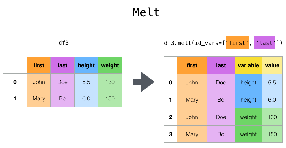
data_loaded_sub_long = data_loaded_sub.melt(id_vars=data_loaded_sub.columns[:5],
                                            value_vars=['movie', 'snack', 'animal'],
                                            var_name='category', value_name='item').drop_duplicates().replace(to_replace='None', value=np.nan).dropna()
data_loaded_sub_long.head(n=10)
| participant | session | age | left-handed | like this course | category | item | |
|---|---|---|---|---|---|---|---|
| 0 | Heidi Klum | 1.0 | 43.0 | False | Yes | movie | The Intouchables |
| 1 | Heidi Klum | 1.0 | 43.0 | False | Yes | movie | James Bond |
| 2 | Heidi Klum | 1.0 | 43.0 | False | Yes | movie | Forrest Gump |
| 3 | Heidi Klum | 1.0 | 43.0 | False | Yes | movie | Retired Extremely Dangerous |
| 4 | Heidi Klum | 1.0 | 43.0 | False | Yes | movie | The Imitation Game |
| 5 | Heidi Klum | 1.0 | 43.0 | False | Yes | movie | The Philosophers |
| 6 | Heidi Klum | 1.0 | 43.0 | False | Yes | movie | Call Me by Your Name |
| 7 | Heidi Klum | 1.0 | 43.0 | False | Yes | movie | Shutter Island |
| 8 | Heidi Klum | 1.0 | 43.0 | False | Yes | movie | Love actually |
| 9 | Heidi Klum | 1.0 | 43.0 | False | Yes | movie | The Great Gatsby |
That worked reasonably well! We only miss the ratings as we didn’t include them during the reshaping. Thus, we will just select them from the old dataframe and then add them to our new dataframe. During the selection of the respective values, we will remove the nans and change the data type to list for easy handling.
ratings = list(data_loaded_sub['rating_movies.response'].dropna()) + \
          list(data_loaded_sub['rating_snacks.response'].dropna()) + \
          list(data_loaded_sub['rating_animals.response'].dropna())
ratings
[4.0,
 7.0,
 3.44,
 4.0,
 6.02,
 4.0,
 4.0,
 5.04,
 6.5600000000000005,
 3.06,
 2.74,
 5.08,
 4.7,
 5.48,
 6.08,
 4.0,
 3.14,
 5.68,
 6.98,
 2.7,
 5.0,
 5.06,
 6.040000000000001,
 5.08,
 5.06,
 5.92,
 4.58,
 4.02,
 5.5,
 2.0,
 3.04,
 7.0,
 7.0,
 7.0,
 5.04,
 6.0,
 4.94,
 4.78]
Now we can simply add this list of ratings to our dataframe via assigning them to a new column. This works comparably to defining new keys and values in dictionaries:

data_loaded_sub_long['ratings'] = ratings
data_loaded_sub_long.head(n=10)
| participant | session | age | left-handed | like this course | category | item | ratings | |
|---|---|---|---|---|---|---|---|---|
| 0 | Heidi Klum | 1.0 | 43.0 | False | Yes | movie | The Intouchables | 4.00 |
| 1 | Heidi Klum | 1.0 | 43.0 | False | Yes | movie | James Bond | 7.00 |
| 2 | Heidi Klum | 1.0 | 43.0 | False | Yes | movie | Forrest Gump | 3.44 |
| 3 | Heidi Klum | 1.0 | 43.0 | False | Yes | movie | Retired Extremely Dangerous | 4.00 |
| 4 | Heidi Klum | 1.0 | 43.0 | False | Yes | movie | The Imitation Game | 6.02 |
| 5 | Heidi Klum | 1.0 | 43.0 | False | Yes | movie | The Philosophers | 4.00 |
| 6 | Heidi Klum | 1.0 | 43.0 | False | Yes | movie | Call Me by Your Name | 4.00 |
| 7 | Heidi Klum | 1.0 | 43.0 | False | Yes | movie | Shutter Island | 5.04 |
| 8 | Heidi Klum | 1.0 | 43.0 | False | Yes | movie | Love actually | 6.56 |
| 9 | Heidi Klum | 1.0 | 43.0 | False | Yes | movie | The Great Gatsby | 3.06 |
Even though this multi-step approach appears a bit cumbersome and introduces more room for errors, the important aspect is that we have everything in code making it reproducible and “easy” to find/spot potential mistakes.
That being said, this might be a good time to save our converted and cleaned dataframe to disk for further analyzes. Importantly, the idea here is that we finished the initial data exploration and wrangling steps for a single participant and can now save the data to avoid running everything again every time we want to work with the data.
Obviously, pandas has our back with the .to_csv() function through which we can just provide a name for the to be saved dataframe resulting in a respective .csv file. (NB: use .to and tab completion to check all other file types you can save your dataframes to.)
from os import makedirs
makedirs('data_experiment/derivatives/preprocessing')
data_loaded_sub_long.to_csv('data_experiment/derivatives/preprocessing/%s_long_format.csv' %data_loaded_sub_long['participant'][0], index=False)
ls data_experiment/derivatives/preprocessing/
Heidi Klum_long_format.csv
While this seems already super intense concerning data analyzes steps, it’s only just the beginning and actually an important aspects focusing on data quality control and preparation of further analyzes. When working with other dataset you might have to less or way more of these operations, depending on a variety of factors.
However, to avoid going through all these steps for each participant, we can simply use our list of data files again and apply all steps within a for loop. Important: only do this if you have your operations outlined and tested, as well as are sure the data doesn’t change between participants.
for index, participant in enumerate(data_files):

    print('Working on %s, file %s/%s' %(participant, index+1, len(data_files)))

    # load the dataframe
    data_loaded_part = pd.read_csv(participant, delimiter=',')

    # select columns
    data_loaded_sub_part = data_loaded_part[columns_select]

    print('Checking for nan across rows and deleting rows with only nan.')

    # create empty list to store NaN rows
    rows_del = []

    # loop through rows and check if they only contain NaN, if so append index to list
    for index, values in data_loaded_sub_part[data_loaded_sub_part.columns[5:]].iterrows():

        if values.isnull().all():
            rows_del.append(index)

    # remove rows that only contain NaN
    data_loaded_sub_part = data_loaded_sub_part.drop(rows_del)

    # reset index
    data_loaded_sub_part.reset_index(drop=True, inplace=True)

    print('Reshaping the dataframe.')

    # bring dataframe to long-format
    data_loaded_sub_part_long = data_loaded_sub_part.melt(id_vars=data_loaded_sub_part.columns[:5],
                                                          value_vars=['movie', 'snack', 'animal'],
                                                          var_name='category', value_name='item').drop_duplicates().replace(to_replace='None', value=np.nan).dropna()
    # exract ratings while removing rows with NaN
    ratings = list(data_loaded_sub_part['rating_movies.response'].dropna()) + \
              list(data_loaded_sub_part['rating_snacks.response'].dropna()) + \
              list(data_loaded_sub_part['rating_animals.response'].dropna())

    # add ratings to long-format dataframe
    data_loaded_sub_part_long['ratings'] = ratings

    print('Saving dataframe to %s_long_format.csv' %data_loaded_sub_part_long['participant'][0])

    # save long-format dataframe
    data_loaded_sub_part_long.to_csv('data_experiment/derivatives/preprocessing/%s_long_format.csv' %data_loaded_sub_part_long['participant'][0], index=False)
Working on data_experiment/yagurllea_experiment_2022_Jan_25_1318.csv, file 1/15
Checking for nan across rows and deleting rows with only nan.
Reshaping the dataframe.
Saving dataframe to yagurllea_long_format.csv
Working on data_experiment/pauli4psychopy_experiment_2022_Jan_24_1145.csv, file 2/15
Checking for nan across rows and deleting rows with only nan.
Reshaping the dataframe.
Saving dataframe to pauli4psychopy_long_format.csv
Working on data_experiment/porla_experiment_2022_Jan_24_2154.csv, file 3/15
Checking for nan across rows and deleting rows with only nan.
Reshaping the dataframe.
Saving dataframe to porla_long_format.csv
Working on data_experiment/Nina__experiment_2022_Jan_24_1212.csv, file 4/15
Checking for nan across rows and deleting rows with only nan.
Reshaping the dataframe.
Saving dataframe to Nina _long_format.csv
Working on data_experiment/Sophie Oprée_experiment_2022_Jan_24_1411.csv, file 5/15
Checking for nan across rows and deleting rows with only nan.
Reshaping the dataframe.
Saving dataframe to Sophie Oprée_long_format.csv
Working on data_experiment/participant_123_experiment_2022_Jan_26_1307.csv, file 6/15
Checking for nan across rows and deleting rows with only nan.
Reshaping the dataframe.
Saving dataframe to participant_123_long_format.csv
Working on data_experiment/funny_ID_experiment_2022_Jan_24_1215.csv, file 7/15
Checking for nan across rows and deleting rows with only nan.
Reshaping the dataframe.
Saving dataframe to funny ID_long_format.csv
Working on data_experiment/Chiara Ferrandina_experiment_2022_Jan_24_1829.csv, file 8/15
Checking for nan across rows and deleting rows with only nan.
Reshaping the dataframe.
Saving dataframe to Chiara Ferrandina_long_format.csv
Working on data_experiment/Smitty_Werben_Jagger_Man_Jensen#1_experiment_2022_Jan_26_1158.csv, file 9/15
Checking for nan across rows and deleting rows with only nan.
Reshaping the dataframe.
Saving dataframe to Smitty_Werben_Jagger_Man_Jensen#1_long_format.csv
Working on data_experiment/wile_coyote_2022_Jan_23_1805.csv, file 10/15
Checking for nan across rows and deleting rows with only nan.
Reshaping the dataframe.
Saving dataframe to wile_coyote_long_format.csv
Working on data_experiment/Heidi_Klum_experiment_2022_Jan_26_1600.csv, file 11/15
Checking for nan across rows and deleting rows with only nan.
Reshaping the dataframe.
Saving dataframe to Heidi Klum_long_format.csv
Working on data_experiment/bugs bunny_experiment_2022_Jan_23_1745.csv, file 12/15
Checking for nan across rows and deleting rows with only nan.
Reshaping the dataframe.
Saving dataframe to bugs_bunny_long_format.csv
Working on data_experiment/Bruce_Wayne_experiment_2022_Jan_23_1605.csv, file 13/15
Checking for nan across rows and deleting rows with only nan.
Reshaping the dataframe.
Saving dataframe to Bruce_Wayne_long_format.csv
Working on data_experiment/twentyfour_experiment_2022_Jan_26_1436.csv, file 14/15
Checking for nan across rows and deleting rows with only nan.
Reshaping the dataframe.
Saving dataframe to Talha_long_format.csv
Working on data_experiment/daffy_duck_experiment_2022_Jan_23_1409.csv, file 15/15
Checking for nan across rows and deleting rows with only nan.
Reshaping the dataframe.
Saving dataframe to daffy_duck_long_format.csv
Yes, the loop looks a bit frightening but it’s really just containing all the necessary steps we explored and we could evaluate potential problems further via the following little print messages.
Let’s check our preprocessed data:
ls data_experiment/derivatives/preprocessing/
Bruce_Wayne_long_format.csv
Chiara Ferrandina_long_format.csv
Heidi Klum_long_format.csv
Nina _long_format.csv
Smitty_Werben_Jagger_Man_Jensen#1_long_format.csv
Sophie Oprée_long_format.csv
Talha_long_format.csv
bugs_bunny_long_format.csv
daffy_duck_long_format.csv
funny ID_long_format.csv
participant_123_long_format.csv
pauli4psychopy_long_format.csv
porla_long_format.csv
wile_coyote_long_format.csv
yagurllea_long_format.csv
The next step of our analyzes would be to combine the single participant dataframes to one group dataframe that contains data from all participants. This will definitely come in handy and is more or less needed for the subsequent steps, including data visualization and statistical analyses.
When it comes to combining dataframes, pandas once more has a variety of options to perform such operations: merge, concat, join and compare, each serving a distinct function. Here, we will use concat to concatenate or stack our dataframes.
For this to work, we need a list of loaded dataframes.
list_dataframes = glob('data_experiment/derivatives/preprocessing/*.csv')

list_dataframes_loaded = []

for dataframe in list_dataframes:

    print('Loading dataframe %s' %dataframe)

    df_part = pd.read_csv(dataframe)

    list_dataframes_loaded.append(df_part)

print('The number of loaded dataframes matches the number of available dataframes: %s'
      %(len(list_dataframes_loaded)==len(list_dataframes)))
Loading dataframe data_experiment/derivatives/preprocessing/Smitty_Werben_Jagger_Man_Jensen#1_long_format.csv
Loading dataframe data_experiment/derivatives/preprocessing/bugs_bunny_long_format.csv
Loading dataframe data_experiment/derivatives/preprocessing/pauli4psychopy_long_format.csv
Loading dataframe data_experiment/derivatives/preprocessing/Heidi Klum_long_format.csv
Loading dataframe data_experiment/derivatives/preprocessing/Sophie Oprée_long_format.csv
Loading dataframe data_experiment/derivatives/preprocessing/daffy_duck_long_format.csv
Loading dataframe data_experiment/derivatives/preprocessing/Nina _long_format.csv
Loading dataframe data_experiment/derivatives/preprocessing/wile_coyote_long_format.csv
Loading dataframe data_experiment/derivatives/preprocessing/funny ID_long_format.csv
Loading dataframe data_experiment/derivatives/preprocessing/yagurllea_long_format.csv
Loading dataframe data_experiment/derivatives/preprocessing/participant_123_long_format.csv
Loading dataframe data_experiment/derivatives/preprocessing/porla_long_format.csv
Loading dataframe data_experiment/derivatives/preprocessing/Chiara Ferrandina_long_format.csv
Loading dataframe data_experiment/derivatives/preprocessing/Bruce_Wayne_long_format.csv
Loading dataframe data_experiment/derivatives/preprocessing/Talha_long_format.csv
The number of loaded dataframes matches the number of available dataframes: True
Now, we can use concat to combine the list of loaded dataframes. (NB: make sure the used combination function matches your use case and is specified correctly re the axis, etc.)
dataframe_concat = pd.concat(list_dataframes_loaded)
dataframe_concat.reset_index(drop=True, inplace=True)
Let’s check what we have:
print('The concatenated dataframe has the following dimensions: %s' %str(dataframe_concat.shape))
print('We have the following columns: %s' %list(dataframe_concat.columns))
print('We have the following participants: %s' %dataframe_concat['participant'].unique())
The concatenated dataframe has the following dimensions: (570, 8)
We have the following columns: ['participant', 'session', 'age', 'left-handed', 'like this course', 'category', 'item', 'ratings']
We have the following participants: ['Smitty_Werben_Jagger_Man_Jensen#1' 'bugs_bunny' 'pauli4psychopy'
 'Heidi Klum' 'Sophie Oprée' 'daffy_duck' 'Nina ' 'wile_coyote' 'funny ID'
 'yagurllea' 'participant_123' 'porla' 'Chiara Ferrandina' 'Bruce_Wayne'
 'Talha']
We can now make use of the .describe() function to get some first insights at the group level.
dataframe_concat.describe()
| session | age | ratings | |
|---|---|---|---|
| count | 570.0 | 570.000000 | 570.000000 |
| mean | 1.0 | 25.866667 | 5.080737 |
| std | 0.0 | 7.326417 | 1.675161 |
| min | 1.0 | 21.000000 | 1.000000 |
| 25% | 1.0 | 22.000000 | 4.000000 |
| 50% | 1.0 | 22.000000 | 5.120000 |
| 75% | 1.0 | 25.000000 | 6.695000 |
| max | 1.0 | 43.000000 | 7.000000 |
However, given the shape and structure of our dataframe we actually might want to consider being more precise and splitting aspects, as we have e.g. multiple entries for each participants age and can’t distinguish ratings based on categories.
Regarding these things, the .groupby() function can be very helpful as it allows us to group and separate our dataframe based on certain aspects, e.g. categories. It will return a form of list with subdataframes given the specified grouping aspect, e.g. category and thus movies, snacks and animals.
for index, df in dataframe_concat.groupby('category'):
    print('Showing information for subdataframe: %s' %index)
    print(df['ratings'].describe())
Showing information for subdataframe: animal
count    90.000000
mean      5.701111
std       1.187184
min       2.400000
25%       4.985000
50%       5.940000
75%       6.980000
max       7.000000
Name: ratings, dtype: float64
Showing information for subdataframe: movie
count    255.000000
mean       4.806118
std        1.795347
min        1.000000
25%        4.000000
50%        5.000000
75%        6.260000
max        7.000000
Name: ratings, dtype: float64
Showing information for subdataframe: snack
count    225.000000
mean       5.143822
std        1.633625
min        1.000000
25%        4.000000
50%        5.680000
75%        6.460000
max        7.000000
Name: ratings, dtype: float64
Comparably, we could use indexing/selecting again to work with respective subdataframes:
dataframe_concat[dataframe_concat['category']=='movie']
| participant | session | age | left-handed | like this course | category | item | ratings | |
|---|---|---|---|---|---|---|---|---|
| 0 | Smitty_Werben_Jagger_Man_Jensen#1 | 1.0 | 42.0 | False | No | movie | The Intouchables | 1.00 |
| 1 | Smitty_Werben_Jagger_Man_Jensen#1 | 1.0 | 42.0 | False | No | movie | James Bond | 1.00 |
| 2 | Smitty_Werben_Jagger_Man_Jensen#1 | 1.0 | 42.0 | False | No | movie | Forrest Gump | 1.00 |
| 3 | Smitty_Werben_Jagger_Man_Jensen#1 | 1.0 | 42.0 | False | No | movie | Retired Extremely Dangerous | 1.00 |
| 4 | Smitty_Werben_Jagger_Man_Jensen#1 | 1.0 | 42.0 | False | No | movie | The Imitation Game | 1.00 |
| ... | ... | ... | ... | ... | ... | ... | ... | ... |
| 544 | Talha | 1.0 | 21.0 | True | Yes | movie | Lord of the Rings - The Two Towers | 6.58 |
| 545 | Talha | 1.0 | 21.0 | True | Yes | movie | Fight Club | 4.98 |
| 546 | Talha | 1.0 | 21.0 | True | Yes | movie | Harry Potter | 2.04 |
| 547 | Talha | 1.0 | 21.0 | True | Yes | movie | Harry Potter and the MatLab-Prince | 1.04 |
| 548 | Talha | 1.0 | 21.0 | True | Yes | movie | Shindlers List | 6.98 |
255 rows × 8 columns
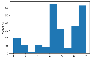
With that, we could start visualizing and analyzing our data via inferential statistics. Regarding the former, pandas even has some built-in functions for basic plotting. Here, some spoilers: a histogram for movie ratings

dataframe_concat[dataframe_concat['category']=='movie']['ratings'].plot.hist()
<AxesSubplot:ylabel='Frequency'>
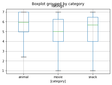
and a boxplot for ratings across categories:
dataframe_concat[['category', 'ratings']].boxplot(by='category')
<AxesSubplot:title={'center':'ratings'}, xlabel='[category]'>
Sorry, but that’s enough spoilers…way more on data visualization next week! For now, we should definitely save the concatenated dataframe as we need it for everything that follows!
dataframe_concat.to_csv('data_experiment/derivatives/preprocessing/dataframe_group.csv', index=False)
Outro/Q&A
What we went through in this session was intended as a super small showcase of working with certain data formats and files in python, specifically using pandas which we only just started to explore and has way more functionality.
Sure: this was a very specific use case and data but the steps and underlying principles are transferable to the majority of data handling/wrangling problems/tasks you might encounter. As always: make sure to check the fantastic docs of the python module you’re using (https://pandas.pydata.org/), as well as all the fantastic tutorials out there.
We can explore its functions via pd. and then using tab completion.
pd.
The core Python “data science” stack
The Python ecosystem contains tens of thousands of packages
Several are very widely used in data science applications:
Jupyter: interactive notebooks
Numpy: numerical computing in Python
pandas: data structures for Python
Scipy: scientific Python tools
Matplotlib: plotting in Python
scikit-learn: machine learning in Python
We’ll cover the first three very briefly here
Other tutorials will go into greater detail on most of the others
The core “Python for psychology” stack
The
Python ecosystemcontains tens of thousands ofpackagesSeveral are very widely used in psychology research:
Jupyter: interactive notebooks
Numpy: numerical computing in
Pythonpandas: data structures for
PythonScipy: scientific
PythontoolsMatplotlib: plotting in
Pythonseaborn: plotting in
Pythonscikit-learn: machine learning in
Pythonstatsmodels: statistical analyses in
Pythonpingouin: statistical analyses in
Pythonpsychopy: running experiments in
Pythonnilearn: brain imaging analyses in `Python``
mne: electrophysiology analyses in
Python
Execept
scikit-learn,nilearnandmne, we’ll cover all very briefly in this coursethere are many free tutorials online that will go into greater detail and also cover the other
packages
Homework assignment #8
Your eight homework assignment will entail working through a few tasks covering the contents discussed in this session within of a jupyter notebook. You can download it here. In order to open it, put the homework assignment notebook within the folder you stored the course materials, start a jupyter notebook as during the sessions, navigate to the homework assignment notebook, open it and have fun!
Deadline: 02/02/2022, 11:59 PM EST