Introduction IV - the jupyter ecosystem & notebooks
Contents
Introduction IV - the jupyter ecosystem & notebooks
Peer Herholz (he/him)
Habilitation candidate - Fiebach Lab, Neurocognitive Psychology at Goethe-University Frankfurt
Research affiliate - NeuroDataScience lab at MNI/McGill
Member - BIDS, ReproNim, Brainhack, Neuromod, OHBM SEA-SIG, UNIQUE
![]()
![]() @peerherholz
@peerherholz
Before we get started 1…
most of what you’ll see within this lecture was prepared by Ross Markello, Michael Notter and Peer Herholz and further adapted for this course by Peer Herholz
based on Tal Yarkoni’s “Introduction to Python” lecture at Neurohackademy 2019
based on http://www.stavros.io/tutorials/python/ & http://www.swaroopch.com/notes/python
based on https://github.com/oesteban/biss2016 & https://github.com/jvns/pandas-cookbook
Objectives 📍
learn basic and efficient usage of the
jupyter ecosystem¬ebookswhat is
Jupyter& how to utilizejupyter notebooks
To Jupyter & beyond

a community of people
an ecosystem of open tools and standards for interactive computing
language-agnostic and modular
empower people to use other open tools
To Jupyter & beyond

Before we get started 2…
We’re going to be working in Jupyter notebooks for most of this presentation!
To load yours, do the following:
Open a terminal/shell & navigate to the folder where you stored the course material (
cd)
Type
jupyter notebook
If you’re not automatically directed to a webpage copy the URL (
https://....) printed in theterminaland paste it in yourbrowser
Files Tab
The files tab provides an interactive view of the portion of the filesystem which is accessible by the user. This is typically rooted by the directory in which the notebook server was started.
The top of the files list displays clickable breadcrumbs of the current directory. It is possible to navigate the filesystem by clicking on these breadcrumbs or on the directories displayed in the notebook list.
A new notebook can be created by clicking on the New dropdown button at the top of the list, and selecting the desired language kernel.
Notebooks can also be uploaded to the current directory by dragging a notebook file onto the list or by clicking the Upload button at the top of the list.
The Notebook
When a notebook is opened, a new browser tab will be created which presents the notebook user interface (UI). This UI allows for interactively editing and running the notebook document.
A new notebook can be created from the dashboard by clicking on the Files tab, followed by the New dropdown button, and then selecting the language of choice for the notebook.
An interactive tour of the notebook UI can be started by selecting Help -> User Interface Tour from the notebook menu bar.
Header
At the top of the notebook document is a header which contains the notebook title, a menubar, and toolbar. This header remains fixed at the top of the screen, even as the body of the notebook is scrolled. The title can be edited in-place (which renames the notebook file), and the menubar and toolbar contain a variety of actions which control notebook navigation and document structure.

Body
The body of a notebook is composed of cells. Each cell contains either markdown, code input, code output, or raw text. Cells can be included in any order and edited at-will, allowing for a large amount of flexibility for constructing a narrative.
Markdown cells- These are used to build anicely formatted narrativearound thecodein the document. The majority of this lesson is composed ofmarkdown cells.to get a
markdown cellyou can either select thecelland useesc+mor viaCell -> cell type -> markdown

Code cells- These are used to define thecomputational codein thedocument. They come intwo forms:the
input cellwhere theusertypes thecodeto beexecuted,and the
output cellwhich is therepresentationof theexecuted code. Depending on thecode, thisrepresentationmay be asimple scalar value, or something more complex like aplotor aninteractive widget.
to get a
code cellyou can either select thecelland useesc+yor viaCell -> cell type -> code
Raw cells- These are used whentextneeds to be included inraw form, withoutexecutionortransformation.
Modality
The notebook user interface is modal. This means that the keyboard behaves differently depending upon the current mode of the notebook. A notebook has two modes: edit and command.
Edit mode is indicated by a green cell border and a prompt showing in the editor area. When a cell is in edit mode, you can type into the cell, like a normal text editor.

Command mode is indicated by a grey cell border. When in command mode, the structure of the notebook can be modified as a whole, but the text in individual cells cannot be changed. Most importantly, the keyboard is mapped to a set of shortcuts for efficiently performing notebook and cell actions. For example, pressing c when in command mode, will copy the current cell; no modifier is needed.

Keyboard Navigation
The modal user interface of the IPython Notebook has been optimized for efficient keyboard usage. This is made possible by having two different sets of keyboard shortcuts: one set that is active in edit mode and another in command mode.
The most important keyboard shortcuts are Enter, which enters edit mode, and Esc, which enters command mode.
In edit mode, most of the keyboard is dedicated to typing into the cell's editor. Thus, in edit mode there are relatively few shortcuts. In command mode, the entire keyboard is available for shortcuts, so there are many more possibilities.
The following images give an overview of the available keyboard shortcuts. These can viewed in the notebook at any time via the Help -> Keyboard Shortcuts menu item.

The following shortcuts have been found to be the most useful in day-to-day tasks:
Basic navigation:
enter,shift-enter,up/k,down/jSaving the
notebook:sCell types:y,m,1-6,rCell creation:a,bCell editing:x,c,v,d,z,ctrl+shift+-Kernel operations:i,.
Markdown Cells
Text can be added to IPython Notebooks using Markdown cells. Markdown is a popular markup language that is a superset of HTML. Its specification can be found here:
http://daringfireball.net/projects/markdown/
You can view the source of a cell by double clicking on it, or while the cell is selected in command mode, press Enter to edit it. Once a cell has been edited, use Shift-Enter to re-render it.
Markdown basics
You can make text italic or bold.
You can build nested itemized or enumerated lists:
One
Sublist
This
Sublist - That - The other thing
Two
Sublist
Three
Sublist
Now another list:
Here we go
Sublist
Sublist
There we go
Now this
You can add horizontal rules:
Here is a blockquote:
Beautiful is better than ugly. Explicit is better than implicit. Simple is better than complex. Complex is better than complicated. Flat is better than nested. Sparse is better than dense. Readability counts. Special cases aren’t special enough to break the rules. Although practicality beats purity. Errors should never pass silently. Unless explicitly silenced. In the face of ambiguity, refuse the temptation to guess. There should be one– and preferably only one –obvious way to do it. Although that way may not be obvious at first unless you’re Dutch. Now is better than never. Although never is often better than right now. If the implementation is hard to explain, it’s a bad idea. If the implementation is easy to explain, it may be a good idea. Namespaces are one honking great idea – let’s do more of those!
You can add headings using Markdown’s syntax:
# Heading 1

# Heading 2

## Heading 2.1

## Heading 2.2
Embedded code
You can embed code meant for illustration instead of execution in Python:
def f(x):
    """a docstring"""
    return x**2
or other languages:
if (i=0; i<n; i++) {
  printf("hello %d\n", i);
  x += 4;
}
Github flavored markdown (GFM)
The Notebook webapp supports Github flavored markdown meaning that you can use triple backticks for code blocks
```python
print "Hello World"
```

```javascript
console.log("Hello World")
```
Gives
print "Hello World"
console.log("Hello World")
And a table like this :
| This | is   |
|------|------|
|   a  | table|
A nice HTML Table
This |
is |
|---|---|
a |
table |
General HTML
Because Markdown is a superset of HTML you can even add things like HTML tables:
| Header 1 | Header 2 |
|---|---|
| row 1, cell 1 | row 1, cell 2 |
| row 2, cell 1 | row 2, cell 2 |
Local files
If you have local files in your Notebook directory, you can refer to these files in Markdown cells directly:
[subdirectory/]<filename>
For example, in the static folder, we have the logo:
<img src="static/pfp_logo.png" />
These do not embed the data into the notebook file, and require that the files exist when you are viewing the notebook.
Security of local files
Note that this means that the IPython notebook server also acts as a generic file server for files inside the same tree as your notebooks. Access is not granted outside the notebook folder so you have strict control over what files are visible, but for this reason it is highly recommended that you do not run the notebook server with a notebook directory at a high level in your filesystem (e.g. your home directory).
When you run the notebook in a password-protected manner, local file access is restricted to authenticated users unless read-only views are active.
Markdown attachments
Since Jupyter notebook version 5.0, in addition to referencing external files you can attach a file to a markdown cell. To do so drag the file from e.g. the browser or local storage in a markdown cell while editing it:

![]()
Files are stored in cell metadata and will be automatically scrubbed at save-time if not referenced. You can recognize attached images from other files by their url that starts with attachment. For the image above:

Keep in mind that attached files will increase the size of your notebook.
You can manually edit the attachement by using the View > Cell Toolbar > Attachment menu, but you should not need to.
Code cells
When executing code in IPython, all valid Python syntax works as-is, but IPython provides a number of features designed to make the interactive experience more fluid and efficient. First, we need to explain how to run cells. Try to run the cell below!
import pandas as pd

print("Hi! This is a cell. Click on it and press the ▶ button above to run it")
Hi! This is a cell. Click on it and press the ▶ button above to run it
You can also run a cell with Ctrl+Enter or Shift+Enter. Experiment a bit with that.
Tab Completion
One of the most useful things about Jupyter Notebook is its tab completion.
Try this: click just after read_csv( in the cell below and press Shift+Tab 4 times, slowly. Note that if you’re using JupyterLab you don’t have an additional help box option.
pd.read_csv(
After the first time, you should see this:

After the second time:

After the fourth time, a big help box should pop up at the bottom of the screen, with the full documentation for the read_csv function:

This is amazingly useful. You can think of this as “the more confused I am, the more times I should press Shift+Tab”.
Okay, let’s try tab completion for function names!
pd.r
You should see this:

Get Help
There’s an additional way on how you can reach the help box shown above after the fourth Shift+Tab press. Instead, you can also use obj? or obj?? to get help or more help for an object.
pd.read_csv?
Writing code
Writing code in a notebook is pretty normal.
def print_10_nums():
    for i in range(10):
        print(i)
print_10_nums()
0
1
2
3
4
5
6
7
8
9
If you messed something up and want to revert to an older version of a code in a cell, use Ctrl+Z or to go than back Ctrl+Y.
For a full list of all keyboard shortcuts, click on the small keyboard icon in the notebook header or click on Help > Keyboard Shortcuts.
The interactive workflow: input, output, history
Notebooks provide various options for inputs and outputs, while also allowing to access the history of run commands.
2+10
12
_+10
22
You can suppress the storage and rendering of output if you append ; to the last cell (this comes in handy when plotting with matplotlib, for example):
10+20;
_
22
The output is stored in _N and Out[N] variables:
_8 == Out[8]
True
Previous inputs are available, too:
In[9]
'_8 == Out[8]'
_i
'In[9]'
%history -n 1-5
   1:
import pandas as pd

print("Hi! This is a cell. Click on it and press the ▶ button above to run it")
   2: pd.read_csv?
   3:
def print_10_nums():
    for i in range(10):
        print(i)
   4: print_10_nums()
   5: 2+10
Accessing the underlying operating system
Through notebooks you can also access the underlying operating system and communicate with it as you would do in e.g. a terminal via bash:
!pwd
/Users/peerherholz/google_drive/GitHub/Python_for_Psychologists_Winter2021/lecture/introduction
files = !ls
print("My current directory's files:")
print(files)
My current directory's files:
['fancy_analyzes.py', 'gui_cli_example_bash.sh', 'gui_cli_example_python.py', 'intro_jupyter.ipynb', 'intro_to_git_and_github.ipynb', 'intro_to_shell.ipynb', 'introduction.md', 'introduction_1.md', 'introduction_2.md', 'introduction_3.md']
!echo $files
[fancy_analyzes.py, gui_cli_example_bash.sh, gui_cli_example_python.py, intro_jupyter.ipynb, intro_to_git_and_github.ipynb, intro_to_shell.ipynb, introduction.md, introduction_1.md, introduction_2.md, introduction_3.md]
!echo {files[0].upper()}
FANCY_ANALYZES.PY
Magic functions
IPython has all kinds of magic functions. Magic functions are prefixed by % or %%, and typically take their arguments without parentheses, quotes or even commas for convenience. Line magics take a single % and cell magics are prefixed with two %%.
Some useful magic functions are:
Magic Name |
Effect |
|---|---|
%env |
Get, set, or list environment variables |
%pdb |
Control the automatic calling of the pdb interactive debugger |
%pylab |
Load numpy and matplotlib to work interactively |
%%debug |
Activates debugging mode in cell |
%%html |
Render the cell as a block of HTML |
%%latex |
Render the cell as a block of latex |
%%sh |
%%sh script magic |
%%time |
Time execution of a Python statement or expression |
You can run %magic to get a list of magic functions or %quickref for a reference sheet.
%magic
Line vs cell magics:
%timeit list(range(1000))
11.6 µs ± 247 ns per loop (mean ± std. dev. of 7 runs, 100000 loops each)
%%timeit
list(range(10))
list(range(100))
1.22 µs ± 9.79 ns per loop (mean ± std. dev. of 7 runs, 1000000 loops each)
Line magics can be used even inside code blocks:
for i in range(1, 5):
    size = i*100
    print('size:', size, end=' ')
    %timeit list(range(size))
size: 100 852 ns ± 23.2 ns per loop (mean ± std. dev. of 7 runs, 1000000 loops each)
size: 200 1.27 µs ± 54.3 ns per loop (mean ± std. dev. of 7 runs, 1000000 loops each)
size: 300 2.05 µs ± 50.4 ns per loop (mean ± std. dev. of 7 runs, 100000 loops each)
size: 400 3.37 µs ± 42.7 ns per loop (mean ± std. dev. of 7 runs, 100000 loops each)
Magics can do anything they want with their input, so it doesn’t have to be valid Python:
%%bash
echo "My shell is:" $SHELL
echo "My disk usage is:"
df -h
My shell is: /bin/bash
My disk usage is:
Filesystem      Size   Used  Avail Capacity iused      ifree %iused  Mounted on
/dev/disk1s1   466Gi   10Gi   50Gi    18%  488411 4881964469    0%   /
devfs          200Ki  200Ki    0Bi   100%     705          0  100%   /dev
/dev/disk1s2   466Gi  394Gi   50Gi    89% 4642743 4877810137    0%   /System/Volumes/Data
/dev/disk1s5   466Gi   11Gi   50Gi    19%      11 4882452869    0%   /private/var/vm
map auto_home    0Bi    0Bi    0Bi   100%       0          0  100%   /System/Volumes/Data/home
Another interesting cell magic: create any file you want locally from the notebook:
%%writefile test.txt
This is a test file!
It can contain anything I want...

And more...
Writing test.txt
!cat test.txt
This is a test file!
It can contain anything I want...

And more...
Let’s see what other magics are currently defined in the system:
%lsmagic
Available line magics:
%alias  %alias_magic  %autoawait  %autocall  %automagic  %autosave  %bookmark  %cat  %cd  %clear  %colors  %conda  %config  %connect_info  %cp  %debug  %dhist  %dirs  %doctest_mode  %ed  %edit  %env  %gui  %hist  %history  %killbgscripts  %ldir  %less  %lf  %lk  %ll  %load  %load_ext  %loadpy  %logoff  %logon  %logstart  %logstate  %logstop  %ls  %lsmagic  %lx  %macro  %magic  %man  %matplotlib  %mkdir  %more  %mv  %notebook  %page  %pastebin  %pdb  %pdef  %pdoc  %pfile  %pinfo  %pinfo2  %pip  %popd  %pprint  %precision  %prun  %psearch  %psource  %pushd  %pwd  %pycat  %pylab  %qtconsole  %quickref  %recall  %rehashx  %reload_ext  %rep  %rerun  %reset  %reset_selective  %rm  %rmdir  %run  %save  %sc  %set_env  %store  %sx  %system  %tb  %time  %timeit  %unalias  %unload_ext  %who  %who_ls  %whos  %xdel  %xmode

Available cell magics:
%%!  %%HTML  %%SVG  %%bash  %%capture  %%debug  %%file  %%html  %%javascript  %%js  %%latex  %%markdown  %%perl  %%prun  %%pypy  %%python  %%python2  %%python3  %%ruby  %%script  %%sh  %%svg  %%sx  %%system  %%time  %%timeit  %%writefile

Automagic is ON, % prefix IS NOT needed for line magics.
Writing latex
Let’s use %%latex to render a block of latex:
%%latex
$$F(k) = \int_{-\infty}^{\infty} f(x) e^{2\pi i k} \mathrm{d} x$$
Running normal Python code: execution and errors
Not only can you input normal Python code, you can even paste straight from a Python or IPython shell session:
>>> # Fibonacci series:
... # the sum of two elements defines the next
... a, b = 0, 1
>>> while b < 10:
...     print(b)
...     a, b = b, a+b
1
1
2
3
5
8
In [1]: for i in range(10):
   ...:     print(i, end=' ')
   ...:
0 1 2 3 4 5 6 7 8 9
And when your code produces errors, you can control how they are displayed with the %xmode magic:
%%writefile mod.py

def f(x):
    return 1.0/(x-1)

def g(y):
    return f(y+1)
Writing mod.py
Now let’s call the function g with an argument that would produce an error:
import mod
mod.g(0)
---------------------------------------------------------------------------
ZeroDivisionError                         Traceback (most recent call last)
<ipython-input-30-81c06c6c0e90> in <module>
      1 import mod
----> 2 mod.g(0)

~/google_drive/GitHub/Python_for_Psychologists_Winter2021/lecture/introduction/mod.py in g(y)
      4
      5 def g(y):
----> 6     return f(y+1)

~/google_drive/GitHub/Python_for_Psychologists_Winter2021/lecture/introduction/mod.py in f(x)
      1
      2 def f(x):
----> 3     return 1.0/(x-1)
      4
      5 def g(y):

ZeroDivisionError: float division by zero
%xmode plain
mod.g(0)
Exception reporting mode: Plain
Traceback (most recent call last):

  File "<ipython-input-31-46ce8a1dbba1>", line 2, in <module>
    mod.g(0)

  File "/Users/peerherholz/google_drive/GitHub/Python_for_Psychologists_Winter2021/lecture/introduction/mod.py", line 6, in g
    return f(y+1)

  File "/Users/peerherholz/google_drive/GitHub/Python_for_Psychologists_Winter2021/lecture/introduction/mod.py", line 3, in f
    return 1.0/(x-1)

ZeroDivisionError: float division by zero
%xmode verbose
mod.g(0)
Exception reporting mode: Verbose
---------------------------------------------------------------------------
ZeroDivisionError                         Traceback (most recent call last)
<ipython-input-32-3f57d27a0745> in <module>
      1 get_ipython().run_line_magic('xmode', 'verbose')
----> 2 mod.g(0)
        global mod.g = <function g at 0x7f81988926a8>

~/google_drive/GitHub/Python_for_Psychologists_Winter2021/lecture/introduction/mod.py in g(y=0)
      4
      5 def g(y):
----> 6     return f(y+1)
        global f = <function f at 0x7f819a58b7b8>
        y = 0

~/google_drive/GitHub/Python_for_Psychologists_Winter2021/lecture/introduction/mod.py in f(x=1)
      1
      2 def f(x):
----> 3     return 1.0/(x-1)
        x = 1
      4
      5 def g(y):

ZeroDivisionError: float division by zero
The default %xmode is “context”, which shows additional context but not all local variables. Let’s restore that one for the rest of our session.
%xmode context
Exception reporting mode: Context
Running code in other languages with special %% magics
%%perl
@months = ("July", "August", "September");
print $months[0];
July
%%ruby
name = "world"
puts "Hello #{name.capitalize}!"
Hello World!
/System/Library/Frameworks/Ruby.framework/Versions/2.6/usr/lib/ruby/2.6.0/universal-darwin19/rbconfig.rb:229: warning: Insecure world writable dir /Users/peerherholz in PATH, mode 040707
Raw Input in the notebook
Since 1.0 the IPython notebook web application supports raw_input which for example allow us to invoke the %debug magic in the notebook:
mod.g(0)
---------------------------------------------------------------------------
ZeroDivisionError                         Traceback (most recent call last)
<ipython-input-36-9fa96bd6b3b6> in <module>
----> 1 mod.g(0)

~/google_drive/GitHub/Python_for_Psychologists_Winter2021/lecture/introduction/mod.py in g(y)
      4
      5 def g(y):
----> 6     return f(y+1)

~/google_drive/GitHub/Python_for_Psychologists_Winter2021/lecture/introduction/mod.py in f(x)
      1
      2 def f(x):
----> 3     return 1.0/(x-1)
      4
      5 def g(y):

ZeroDivisionError: float division by zero
%debug
> /Users/peerherholz/google_drive/GitHub/Python_for_Psychologists_Winter2021/lecture/introduction/mod.py(3)f()
      1
      2 def f(x):
----> 3     return 1.0/(x-1)
      4
      5 def g(y):

ipdb> exit()
Don’t forget to exit your debugging session. Raw input can of course be used to ask for user input:
enjoy = input('Are you enjoying this tutorial? ')
print('enjoy is:', enjoy)
Are you enjoying this tutorial? only the snacks
enjoy is: only the snacks
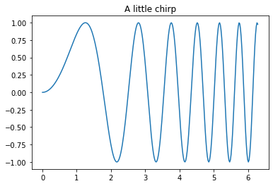
Plotting in the notebook
Notebooks support a variety of fantastic plotting options, including static and interactive graphics. This magic configures matplotlib to render its figures inline:
%matplotlib inline
import numpy as np
import matplotlib.pyplot as plt
x = np.linspace(0, 2*np.pi, 300)
y = np.sin(x**2)
plt.plot(x, y)
plt.title("A little chirp")
fig = plt.gcf()  # let's keep the figure object around for later...
import plotly.figure_factory as ff

# Add histogram data
x1 = np.random.randn(200) - 2
x2 = np.random.randn(200)
x3 = np.random.randn(200) + 2
x4 = np.random.randn(200) + 4

# Group data together
hist_data = [x1, x2, x3, x4]

group_labels = ['Group 1', 'Group 2', 'Group 3', 'Group 4']

# Create distplot with custom bin_size
fig = ff.create_distplot(hist_data, group_labels, bin_size=.2)
fig.show()
The IPython kernel/client model
%connect_info
{
  "shell_port": 60588,
  "iopub_port": 60589,
  "stdin_port": 60590,
  "control_port": 60592,
  "hb_port": 60591,
  "ip": "127.0.0.1",
  "key": "812112ff-f84b0658089eed0149a24418",
  "transport": "tcp",
  "signature_scheme": "hmac-sha256",
  "kernel_name": ""
}

Paste the above JSON into a file, and connect with:
    $> jupyter <app> --existing <file>
or, if you are local, you can connect with just:
    $> jupyter <app> --existing kernel-55f10c28-d38e-452f-b5fa-6002071b8179.json
or even just:
    $> jupyter <app> --existing
if this is the most recent Jupyter kernel you have started.
We can connect automatically a Qt Console to the currently running kernel with the %qtconsole magic, or by typing ipython console --existing <kernel-UUID> in any terminal:
%qtconsole
Saving a Notebook
Jupyter Notebooks autosave, so you don’t have to worry about losing code too much. At the top of the page you can usually see the current save status:
Last Checkpoint: 2 minutes ago (unsaved changes)
Last Checkpoint: a few seconds ago (autosaved)
If you want to save a notebook on purpose, either click on File > Save and Checkpoint or press Ctrl+S.
To Jupyter & beyond
Open a terminal
Type
jupyter lab
If you’re not automatically directed to a webpage copy the URL printed in the terminal and paste it in your browser
Click “New” in the top-right corner and select “Python 3”
You have a
Jupyter notebookwithinJupyter lab!
Homework assignment #2
your second homework assignment will entail the generation of a
jupyter notebookwithmandatory:
3 different cells: - 1 rendered markdown cell within which you name your favorite movie and describe why you like it via
max. 2 sentences - 1 code cell with an equation (e.g.1+1,(a+b)/(c+d), etc.) - 1 raw cell with your favorite snackoptional: try to include a picture of your favorite animal
save the notebook and e-mail it to Peer
deadline: 17/11/2021, 11:59 PM EST