Connectivity analysis - correlation analyses - ROI to ROI
Within this section of the connectivity analyses the ROI to ROI correlation are shown, explained and set up in a way that they can be rerun and reproduced. In short, we employed task-based functional connectivity through NiBetaSeries analysis, to investigate if condition specific information flow between the ROIs of the auditory cortex provides insights concerning the proposed functional principles. The analysis is divided into the following sections:
Correlation analysis - ROI to ROI
Condition-specific functional connectivity
Comparison of condition-specific functional connectivity
We provide more detailed information and explanations in the respective sections. As mentioned before, we’re working with derivatives here and thus we can share them, meaning that you can rerun the analyses either by downloading this page as a Jupyter Notebook (via the download button at the top) or interactively via a cloud instance through the amazing mybinder project (the little rocket at the top). We recommend the later to spare installation and conda environment related problems. One more thing… Please note, that here derivatives refers to the computed Beta Series (i.e. condition specific trial-wise beta estimates) which we provide via the project’s OSF page because their computation is computationally very expensive and would never run via the resources available through binder. The code that will download the required data is included in the respective sections.
As usual, we will start with importing all necessary modules and functions.
from os.path import join as opj
from os.path import basename as opb
from os import listdir
from copy import deepcopy
import numpy as np
from glob import glob
import pandas as pd
import nibabel as nb
from nilearn.connectome import ConnectivityMeasure
from nilearn.input_data import NiftiLabelsMasker
from netneurotools import stats as nnstats
from pingouin import multicomp
import matplotlib.pyplot as plt
from matplotlib.lines import Line2D
import seaborn as sns
import ptitprince as pt
import plotly.express as px
import plotly.graph_objects as go
from IPython.core.display import display, HTML
from plotly.offline import init_notebook_mode, plot
import pingouin as pg
from utils import plot_auditory_cortex_connectome
%matplotlib inline
Let’s also gather and set some important paths. This includes the path to the general derivatives directory, as well as analyses specific ones. In more detail, we of course aim to keep it as BIDS-y as possible and therefore set a path for the Connectivity analyses here. To keep results and necessary prerequisites separate (keeping it tidy), we also create a dedicated directory which will include the auditory cortex atlas, as well as the input data.
derivatives_path = '/data/mvs/derivatives/'
roi_mask_path ='/data/mvs/derivatives/ROIs_masks/'
prereq_path = '/data/mvs/derivatives/connectivity/prerequisites/'
results_path = '/data/mvs/derivatives/connectivity/'
At first, we need to gather the outputs from the previous step, i.e. the computation of Beta Series. Please note: if you want to run this interactively but did not download the Beta Series in the previous step, you need to download them now via this command:
osf -p <projectid> fetch remote/path.txt local/file.txt
What we have as output are betaseries files per condition and run, each containing n images where n reflects the number of presentations of a given condition per run. Thus, we have six betaseries: for each of two runs, one for music, singing and voice respectively.
listdir(opj(results_path, 'nibetaseries_transform/sub-01'))
['sub-01_task-mvs_run-2_space-individual_desc-Singing_betaseries.nii.gz',
'sub-01_task-mvs_run-1_space-individual_desc-Music_betaseries.nii.gz',
'sub-01_task-mvs_run-1_space-individual_desc-Singing_betaseries.nii.gz',
'sub-01_task-mvs_run-2_space-individual_desc-Music_betaseries.nii.gz',
'sub-01_task-mvs_run-1_space-individual_desc-Voice_betaseries.nii.gz',
'sub-01_task-mvs_run-2_space-individual_desc-Voice_betaseries.nii.gz']
And each betaseries consists of 30 images which matches with how often the conditions were presented:
list_beta = glob(opj(results_path, 'nibetaseries_transform/*/*.nii.gz'))
list_beta.sort()
for betaseries in list_beta:
print(nb.load(betaseries).shape)
(97, 115, 97, 30)
(97, 115, 97, 30)
(97, 115, 97, 30)
(97, 115, 97, 30)
(97, 115, 97, 30)
(97, 115, 97, 30)
(97, 115, 97, 30)
(97, 115, 97, 30)
(97, 115, 97, 30)
(97, 115, 97, 30)
(97, 115, 97, 30)
(97, 115, 97, 30)
(97, 115, 97, 30)
(97, 115, 97, 30)
(97, 115, 97, 30)
(97, 115, 97, 30)
(97, 115, 97, 30)
(97, 115, 97, 30)
(97, 115, 97, 30)
(97, 115, 97, 30)
(97, 115, 97, 30)
(97, 115, 97, 30)
(97, 115, 97, 30)
(97, 115, 97, 30)
(97, 115, 97, 30)
(97, 115, 97, 30)
(97, 115, 97, 30)
(97, 115, 97, 30)
(97, 115, 97, 30)
(97, 115, 97, 30)
(97, 115, 97, 30)
(97, 115, 97, 30)
(97, 115, 97, 30)
(97, 115, 97, 30)
(97, 115, 97, 30)
(97, 115, 97, 30)
(97, 115, 97, 30)
(97, 115, 97, 30)
(97, 115, 97, 30)
(97, 115, 97, 30)
(97, 115, 97, 30)
(97, 115, 97, 30)
(97, 115, 97, 30)
(97, 115, 97, 30)
(97, 115, 97, 30)
(97, 115, 97, 30)
(97, 115, 97, 30)
(97, 115, 97, 30)
(97, 115, 97, 30)
(97, 115, 97, 30)
(97, 115, 97, 30)
(97, 115, 97, 30)
(97, 115, 97, 30)
(97, 115, 97, 30)
(97, 115, 97, 30)
(97, 115, 97, 30)
(97, 115, 97, 30)
(97, 115, 97, 30)
(97, 115, 97, 30)
(97, 115, 97, 30)
(97, 115, 97, 30)
(97, 115, 97, 30)
(97, 115, 97, 30)
(97, 115, 97, 30)
(97, 115, 97, 30)
(97, 115, 97, 30)
(97, 115, 97, 30)
(97, 115, 97, 30)
(97, 115, 97, 30)
(97, 115, 97, 30)
(97, 115, 97, 30)
(97, 115, 97, 30)
(97, 115, 97, 30)
(97, 115, 97, 30)
(97, 115, 97, 30)
(97, 115, 97, 30)
(97, 115, 97, 30)
(97, 115, 97, 30)
(97, 115, 97, 30)
(97, 115, 97, 30)
(97, 115, 97, 30)
(97, 115, 97, 30)
(97, 115, 97, 30)
(97, 115, 97, 30)
(97, 115, 97, 30)
(97, 115, 97, 30)
(97, 115, 97, 30)
(97, 115, 97, 30)
(97, 115, 97, 30)
(97, 115, 97, 30)
(97, 115, 97, 30)
(97, 115, 97, 30)
(97, 115, 97, 30)
(97, 115, 97, 30)
(97, 115, 97, 30)
(97, 115, 97, 30)
(97, 115, 97, 30)
(97, 115, 97, 30)
(97, 115, 97, 30)
(97, 115, 97, 30)
(97, 115, 97, 30)
(97, 115, 97, 30)
(97, 115, 97, 30)
(97, 115, 97, 30)
(97, 115, 97, 30)
(97, 115, 97, 30)
(97, 115, 97, 30)
(97, 115, 97, 30)
(97, 115, 97, 30)
(97, 115, 97, 30)
(97, 115, 97, 30)
(97, 115, 97, 30)
(97, 115, 97, 30)
(97, 115, 97, 30)
(97, 115, 97, 30)
(97, 115, 97, 30)
(97, 115, 97, 30)
(97, 115, 97, 30)
(97, 115, 97, 30)
(97, 115, 97, 30)
(97, 115, 97, 30)
(97, 115, 97, 30)
(97, 115, 97, 30)
(97, 115, 97, 30)
(97, 115, 97, 30)
(97, 115, 97, 30)
(97, 115, 97, 30)
(97, 115, 97, 30)
(97, 115, 97, 30)
(97, 115, 97, 30)
(97, 115, 97, 30)
(97, 115, 97, 30)
(97, 115, 97, 30)
(97, 115, 97, 30)
(97, 115, 97, 30)
(97, 115, 97, 30)
(97, 115, 97, 30)
(97, 115, 97, 30)
(97, 115, 97, 30)
(97, 115, 97, 30)
(97, 115, 97, 30)
(97, 115, 97, 30)
(97, 115, 97, 30)
(97, 115, 97, 30)
We can double check the number of presentations of a given condition using sub-01 and the music condition as an example:
pd.read_csv('/data/mvs/sub-01/func/sub-01_task-mvs_run-01_events.tsv', sep='\t').query('trial_type == "Music"').trial_type.count()
30
As done in the MVPA, we will exclude the data of sub-06 as no reliable activation could be detected in the univariate analyses:
del list_beta[30:36]
We just need one more thing to start our analyses: the Auditory cortex atlas information indicating which index is which region. We created this file in the previous step and can now just load it:
atlas_rois_df = pd.read_csv(opj(prereq_path, 'atlas/AC_atlas_regions.txt'), sep='\t')
atlas_rois_df
| index | regions | |
|---|---|---|
| 0 | 1 | HG_lh |
| 1 | 2 | HG_rh |
| 2 | 3 | PP_lh |
| 3 | 4 | PP_rh |
| 4 | 5 | PT_lh |
| 5 | 6 | PT_rh |
| 6 | 7 | aSTG_lh |
| 7 | 8 | aSTG_rh |
| 8 | 9 | pSTG_lh |
| 9 | 10 | pSTG_rh |
Correlation analyses - ROI to ROI
At first, we will compute condition specific connectivity matrices for each run and participant. That is, we are going to assess the correlation of condition specific beta series between the ROIs of our auditory cortex model across time, here trials or presentations. Subsequently, we will compare the resulting connectivity matrices between conditions to evaluate if the information flow diverges between conditions and if so, where. However, before we do so, we need to talk about our auditory cortex model again. In the way we set it up before, it is fully connected, which means that every ROI is connected to every other ROI. Even though we focus on functional principles, it is still important to incorporate results from prior studies concerning both structure and function to evaluate which of our connections actually make sense/are justifiable. Doing so, for example here, here and here, points to a few connections we should keep and quite a bunch we should not keep.
network_structure_reduced = np.array([[0., 2., 1., 0., 1., 0., 0., 0., 0., 0.],
[2., 0., 0., 1., 0., 1., 0., 0., 0., 0.],
[1., 0., 0., 0., 0., 0., 1., 0., 0., 0.],
[0., 1., 0., 0., 0., 0., 0., 1., 0., 0.],
[1., 0., 0., 0., 0., 2., 0., 0., 1., 0.],
[0., 1., 0., 0., 2., 0., 0., 0., 0., 1.],
[0., 0., 1., 0., 0., 0., 0., 0., 0., 0.],
[0., 0., 0., 1., 0., 0., 0., 0., 0., 0.],
[0., 0., 0., 0., 1., 0., 0., 0., 0., 2.],
[0., 0., 0., 0., 0., 1., 0., 0., 2., 0.]])
And we plot it using the function we defined in the previous step:
plot_auditory_cortex_connectome(network_structure_reduced, atlas_info=atlas_rois_df, name='reduced', n_lines=10)
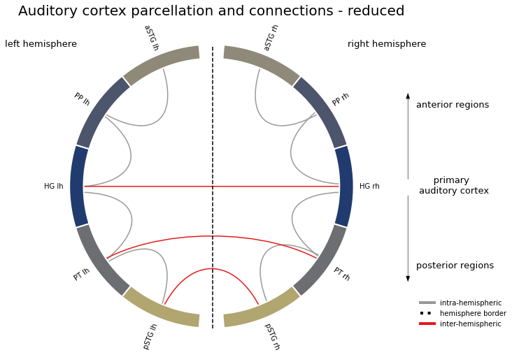
Looks quite different from our fully connected model and while it might seem drastic, cutting the connections down to those that are plausible makes sense.
Condition specific functional connectivity
In order to compute the condition specific functional connectivity between ROIs, we need to do two things: extract the respective beta series for each condition and ROI and subsequently assess the correlation between the beta series of all pairs of ROIs. For the first, we can use nilearn’s NiftiMapsMasker:
masker = NiftiLabelsMasker(opj(results_path,
'prerequisites/atlas/tpl-MNI152NLin2009cAsym_res-02_desc-ACatlas.nii.gz'),
memory='nilearn_cache', standardize=True)
We then create list for the extracted time series and their respective information (participant, run and condition) as we need this for the statistical analysis.
beta_series = []
participant = []
run = []
condition = []
Let’s briefly check if we have all the beta series images we need:
print('We have a total of %s beta series images.' %str(int(len(list_beta))))
print('Given that we have beta series images for 3 conditions and 2 runs each, this means we have data from %s participants.' %str(int(len(list_beta)/(3*2))))
We have a total of 138 beta series images.
Given that we have beta series images for 3 conditions and 2 runs each, this means we have data from 23 participants.
Nice, that checks out. Having everything in place, we can put it together in a loop and extract the beta series, participant id, run and condition:
for betaseries in list_beta:
beta_series.append(masker.fit_transform(betaseries))
participant.append(betaseries[betaseries.rfind('sub'):betaseries.rfind('_task')])
run.append(betaseries[betaseries.rfind('run'):betaseries.rfind('_s')])
condition.append(betaseries[betaseries.rfind('-')+1:betaseries.rfind('_')])
For the ease of use, we put the extracted participant. run and condition information in a DataFrame:
beta_series_info = pd.DataFrame({'participant': participant, 'run': run, 'condition': condition})
beta_series_info.head()
| participant | run | condition | |
|---|---|---|---|
| 0 | sub-01 | run-1 | Music |
| 1 | sub-01 | run-1 | Singing |
| 2 | sub-01 | run-1 | Voice |
| 3 | sub-01 | run-2 | Music |
| 4 | sub-01 | run-2 | Singing |
With that, we can now easily check if we everything worked as expected, including the number and ids of participants:
print('We have a total of %s participants, comprising the following ids: ' %str(int(len(beta_series_info['participant'].unique()))))
list(beta_series_info['participant'].unique())
We have a total of 23 participants, comprising the following ids:
['sub-01',
'sub-02',
'sub-03',
'sub-04',
'sub-05',
'sub-07',
'sub-08',
'sub-09',
'sub-10',
'sub-11',
'sub-12',
'sub-13',
'sub-14',
'sub-15',
'sub-16',
'sub-17',
'sub-18',
'sub-19',
'sub-20',
'sub-21',
'sub-22',
'sub-23',
'sub-24']
and the runs:
print('We have the following runs: ')
print(list(beta_series_info['run'].unique()))
print('(%s in total, 2 for each of 23 participants)' %str(int(len(beta_series_info['participant'].unique()) * len(beta_series_info['run'].unique()))))
We have the following runs:
['run-1', 'run-2']
(46 in total, 2 for each of 23 participants)
and the conditions:
print('We have the following conditions: ')
print(list(beta_series_info['condition'].unique()))
print('(%s in total, 3 for each of 23 participants and 2 runs)' %str(int(len(beta_series_info['participant'].unique()) *
len(beta_series_info['condition'].unique()) *
len(beta_series_info['run'].unique()))))
We have the following conditions:
['Music', 'Singing', 'Voice']
(138 in total, 3 for each of 23 participants and 2 runs)
Great, that looks about right. Next, we are going to add an additional variable to our information DataFrame to enable certain statistical models later on. This refers to a combination of the participant, run and conditions:
list_mod_ind = []
for i, row in beta_series_info.iterrows():
list_mod_ind.append(row['participant']+'_'+row['run']+'_'+row['condition'])
beta_series_info['mod_ind'] = list_mod_ind
Did that work?
beta_series_info.head()
| participant | run | condition | mod_ind | |
|---|---|---|---|---|
| 0 | sub-01 | run-1 | Music | sub-01_run-1_Music |
| 1 | sub-01 | run-1 | Singing | sub-01_run-1_Singing |
| 2 | sub-01 | run-1 | Voice | sub-01_run-1_Voice |
| 3 | sub-01 | run-2 | Music | sub-01_run-2_Music |
| 4 | sub-01 | run-2 | Singing | sub-01_run-2_Singing |
It did! Let’s save these outputs so that we can load them later without having the necessity to rerun the extraction again:
np.save(opj(results_path, 'results/nibetaseries/nibetaseries_transform/beta_series/mss_beta_series.npy'), beta_series, allow_pickle=True)
beta_series_info.to_csv(opj(results_path, 'results/nibetaseries/nibetaseries_transform/beta_series/mvs_beta_series_info.csv'), index=False)
Depending on what and how folks might run the analyses, we will also include code to download this data from the project’s OSF page and load it:
osf -p <projectid> fetch remote/path.txt local/file.txt
beta_series = np.load(opj(results_path, 'results/nibetaseries/nibetaseries_transform/beta_series/mss_beta_series.npy'), allow_pickle=True)
beta_series_info = pd.read_csv(opj(results_path, 'results/nibetaseries/nibetaseries_transform/beta_series/mvs_time_series_info.csv'))
Now we stack the beta series of the two runs for a given condition and participant, also changing the order of conditions to Voice, Singing and Music for consistency reasons. This was motivated by the analyses we wanted to conduct and are outlined further below. We set a few new lists:
part_list = []
cond_list = []
bs_list = []
and iterate over participants and conditions, concatenating beta series across runs:
for part in beta_series_info['participant'].unique():
for cond in ['Voice', 'Singing', 'Music']:
part_list.append(part)
cond_list.append(cond)
bs_list.append(np.vstack(np.array(beta_series)[beta_series_info.condition.isin([cond]) & beta_series_info.participant.isin([part])]))
part_cond = [(part+'_'+cond) for part,cond in zip(part_list, cond_list)]
Let’s create a new DataFrame that reflects those changes:
beta_series_info_stacked = pd.DataFrame({'participant': part_list, 'condition': cond_list, 'part_cond': part_cond})
beta_series_info_stacked.head()
| participant | condition | part_cond | |
|---|---|---|---|
| 0 | sub-01 | Voice | sub-01_Voice |
| 1 | sub-01 | Singing | sub-01_Singing |
| 2 | sub-01 | Music | sub-01_Music |
| 3 | sub-02 | Voice | sub-02_Voice |
| 4 | sub-02 | Singing | sub-02_Singing |
We will also save the stacked versions of the beta series and DataFrame. Please note, that going forward, we will work with the stacked versions only.
np.save(opj(results_path, 'results/nibetaseries/nibetaseries_transform/beta_series/mss_beta_series_desc-stacked.npy'), bs_list, allow_pickle=True)
beta_series_info_stacked.to_csv(opj(results_path, 'results/nibetaseries/nibetaseries_transform/beta_series/mvs_beta_series_info_desc-stacked.csv'), index=False)
We finally arrived at the second step of the ROI to ROI correlation analyses: computing the correlation of beta series between ROIs. Once more, nilearn has our back and we can its ConnectivityMeasure class which makes the computation of connectivity matrices straightforward. First, we need to define our correlation measure. We decided to go with the full correlation following the NiBetaSeries workflow and prior research.
cor_measure = ConnectivityMeasure(kind='correlation')
Second, we apply or fit it to the extracted beta series:
cor_matrices = cor_measure.fit_transform(bs_list, )
This results in n connectivity matrices, one for each condition and participant, thus 69 in total:
cor_matrices.shape
(69, 10, 10)
As you can see each of our 69 connectivity matrices is 10 x 10, this is because our auditory cortex model has 10 regions and thus will always results in the fully connected model. The reduced model we introduced above, will be used to masked those connections that were cut. We will achieve this via a for-loop within which we will set the respective connections of the computed correlation matrices to 0:
for matrix in cor_matrices:
matrix[network_structure_reduced == 0] = int(0)
Let’s check if this worked by comparing our reduced model to one of the masked correlation matrices we just obtained:
network_structure_reduced_viz_test = deepcopy(network_structure_reduced)
network_structure_reduced_viz_test[network_structure_reduced==0] = np.nan
At first, the reduced network model:
fig = px.imshow(network_structure_reduced_viz_test, x=atlas_rois_df['regions'], y=atlas_rois_df['regions'],
color_continuous_scale=['gray', 'red'])
fig.update_layout(coloraxis_showscale=False)
fig['layout'].update(plot_bgcolor='white')
init_notebook_mode(connected=True)
plot(fig, filename = 'ac_network_model_reduced.html')
display(HTML('ac_network_model_reduced.html'))
And as an example, the correlation matrix for the condition voice of sub-01:
cor_matrix_viz_test = cor_matrices[0]
cor_matrix_viz_test[cor_matrices[0]==0] = np.nan
fig = px.imshow(cor_matrix_viz_test, x=atlas_rois_df['regions'], y=atlas_rois_df['regions'],
color_continuous_scale='darkmint_r')
fig.update_layout(coloraxis_showscale=True)
fig['layout'].update(plot_bgcolor='white')
plot(fig, filename = 'ac_network_cor-voice_sub-01.html')
display(HTML('ac_network_cor-voice_sub-01.html'))
A bit hard to see, but using NumPy’s nonzero function we can easily get and compare the indices of values that are not zero:
np.nonzero(network_structure_reduced)
(array([0, 0, 0, 1, 1, 1, 2, 2, 3, 3, 4, 4, 4, 5, 5, 5, 6, 7, 8, 8, 9, 9]),
array([1, 2, 4, 0, 3, 5, 0, 6, 1, 7, 0, 5, 8, 1, 4, 9, 2, 3, 4, 9, 5, 8]))
np.nonzero(cor_matrices[0])
(array([0, 0, 0, 1, 1, 1, 2, 2, 3, 3, 4, 4, 4, 5, 5, 5, 6, 7, 8, 8, 9, 9]),
array([1, 2, 4, 0, 3, 5, 0, 6, 1, 7, 0, 5, 8, 1, 4, 9, 2, 3, 4, 9, 5, 8]))
Ok, things work as expected, cool. Now we will bring the correlation values into a form which makes handling, saving and statistical analyses a bit easier: a Pandas DataFrame. To make this straightforward and because we deal with task-based functional connectivity (thus having a network structure/connectivity matrix that is mirrored across the diagonal), we define a mask that entails the indices of non-zero values of the lower triangle of the network structure/connectivity matrix. Otherwise, we would have the value for each connection twice and this would obscure our planned analyses.
connection_analyses_indices = np.where(np.tril(cor_matrices[0]) != 0)
And to be sure, we check the mask using the example from above:
cor_matrices[0][connection_analyses_indices]
array([0.72974441, 0.73035626, 0.63890314, 0.83369683, 0.75232852,
0.74362356, 0.67876427, 0.42367251, 0.67637752, 0.67960324,
0.77169163])
Fantastic! Now we create a list that specifies which index is which connection to include it into the DataFrame and thus ease that part up a bit:
list_connections = ['HG_lh_HG_rh', 'HG_lh_PP_lh', 'HG_rh_PP_rh', 'HG_lh_PT_lh', 'HG_rh_PT_rh',
'PT_lh_PT_rh', 'PP_lh_aSTG_lh', 'PP_rh_aSTG_rh', 'PT_lh_pSTG_lh', 'PT_rh_pSTG_rh',
'pSTG_lh_pSTG_rh']
Following this order, we are now going to extract the corresponding for a given connection. To do so we will use a combination of list comprehension and indexing which which we will extract a certain connection:
list_HG_lh_HG_rh = [m[connection_analyses_indices][0] for m in cor_matrices]
list_HG_lh_PP_lh = [m[connection_analyses_indices][1] for m in cor_matrices]
list_HG_rh_PP_rh = [m[connection_analyses_indices][2] for m in cor_matrices]
list_HG_lh_PT_lh = [m[connection_analyses_indices][3] for m in cor_matrices]
list_HG_rh_PT_rh = [m[connection_analyses_indices][4] for m in cor_matrices]
list_PT_lh_PT_rh = [m[connection_analyses_indices][5] for m in cor_matrices]
list_PP_lh_aSTG_lh = [m[connection_analyses_indices][6] for m in cor_matrices]
list_PP_rh_aSTG_rh = [m[connection_analyses_indices][7] for m in cor_matrices]
list_PT_lh_pSTG_lh = [m[connection_analyses_indices][8] for m in cor_matrices]
list_PT_rh_pSTG_rh = [m[connection_analyses_indices][9] for m in cor_matrices]
list_pSTG_lh_pSTG_rh = [m[connection_analyses_indices][10] for m in cor_matrices]
With that, we can create our DataFrame. As we already have a lot of useful information in our beta_series_information DataFrame, including participant and run ID, as well as conditions, we will use it as a base:
con_info = deepcopy(beta_series_info_stacked)
and add simply add the extracted correlation values for all connections:
con_info['HG_lh_HG_rh'] = list_HG_lh_HG_rh
con_info['HG_lh_PP_lh'] = list_HG_lh_PP_lh
con_info['HG_rh_PP_rh'] = list_HG_rh_PP_rh
con_info['HG_lh_PT_lh'] = list_HG_lh_PT_lh
con_info['HG_rh_PT_rh'] = list_HG_rh_PT_rh
con_info['PT_lh_PT_rh'] = list_PT_lh_PT_rh
con_info['PP_lh_aSTG_lh'] = list_PP_lh_aSTG_lh
con_info['PP_rh_aSTG_rh'] = list_PP_rh_aSTG_rh
con_info['PT_lh_pSTG_lh'] = list_PT_lh_pSTG_lh
con_info['PT_rh_pSTG_rh'] = list_PT_rh_pSTG_rh
con_info['pSTG_lh_pSTG_rh'] = list_pSTG_lh_pSTG_rh
We now have one big DataFrame with everything we need to run the planned statistical analyses:
con_info
| participant | condition | part_cond | HG_lh_HG_rh | HG_lh_PP_lh | HG_rh_PP_rh | HG_lh_PT_lh | HG_rh_PT_rh | PT_lh_PT_rh | PP_lh_aSTG_lh | PP_rh_aSTG_rh | PT_lh_pSTG_lh | PT_rh_pSTG_rh | pSTG_lh_pSTG_rh | |
|---|---|---|---|---|---|---|---|---|---|---|---|---|---|---|
| 0 | sub-01 | Voice | sub-01_Voice | 0.729744 | 0.730356 | 0.638903 | 0.833697 | 0.752329 | 0.743624 | 0.678764 | 0.423673 | 0.676378 | 0.679603 | 0.771692 |
| 1 | sub-01 | Singing | sub-01_Singing | 0.675542 | 0.771575 | 0.663902 | 0.819895 | 0.722174 | 0.753315 | 0.720142 | 0.531696 | 0.653344 | 0.651568 | 0.687224 |
| 2 | sub-01 | Music | sub-01_Music | 0.664941 | 0.777863 | 0.755443 | 0.864224 | 0.749391 | 0.811263 | 0.671052 | 0.443218 | 0.708958 | 0.620904 | 0.821649 |
| 3 | sub-02 | Voice | sub-02_Voice | 0.830138 | 0.877590 | 0.820580 | 0.855173 | 0.820108 | 0.883193 | 0.689591 | 0.701428 | 0.743975 | 0.789122 | 0.814807 |
| 4 | sub-02 | Singing | sub-02_Singing | 0.781083 | 0.761344 | 0.765417 | 0.737433 | 0.782925 | 0.851739 | 0.582042 | 0.740368 | 0.730446 | 0.756289 | 0.859267 |
| 5 | sub-02 | Music | sub-02_Music | 0.823370 | 0.846985 | 0.785204 | 0.847632 | 0.825368 | 0.869806 | 0.575630 | 0.694261 | 0.696670 | 0.702350 | 0.835517 |
| 6 | sub-03 | Voice | sub-03_Voice | 0.875702 | 0.739229 | 0.746251 | 0.870731 | 0.788325 | 0.868515 | 0.650099 | 0.674626 | 0.810724 | 0.787583 | 0.827930 |
| 7 | sub-03 | Singing | sub-03_Singing | 0.838800 | 0.783068 | 0.798430 | 0.895312 | 0.790128 | 0.860714 | 0.675208 | 0.595846 | 0.847480 | 0.803247 | 0.766505 |
| 8 | sub-03 | Music | sub-03_Music | 0.870248 | 0.827551 | 0.826401 | 0.888271 | 0.835686 | 0.886036 | 0.795027 | 0.792858 | 0.881290 | 0.831516 | 0.866635 |
| 9 | sub-04 | Voice | sub-04_Voice | 0.661841 | 0.669932 | 0.732870 | 0.813031 | 0.653174 | 0.724992 | 0.698228 | 0.730935 | 0.720296 | 0.672631 | 0.735072 |
| 10 | sub-04 | Singing | sub-04_Singing | 0.730157 | 0.702212 | 0.706484 | 0.787749 | 0.768039 | 0.802235 | 0.625223 | 0.634347 | 0.714656 | 0.702342 | 0.780434 |
| 11 | sub-04 | Music | sub-04_Music | 0.724174 | 0.691277 | 0.694784 | 0.806611 | 0.749147 | 0.814798 | 0.709694 | 0.788474 | 0.744303 | 0.781017 | 0.770780 |
| 12 | sub-05 | Voice | sub-05_Voice | 0.897685 | 0.807468 | 0.810559 | 0.909669 | 0.882354 | 0.910752 | 0.797057 | 0.560030 | 0.785998 | 0.836483 | 0.889023 |
| 13 | sub-05 | Singing | sub-05_Singing | 0.799600 | 0.752605 | 0.692251 | 0.876613 | 0.798767 | 0.868799 | 0.699611 | 0.650478 | 0.801587 | 0.848003 | 0.888526 |
| 14 | sub-05 | Music | sub-05_Music | 0.865606 | 0.813042 | 0.783262 | 0.883580 | 0.819614 | 0.856640 | 0.760175 | 0.585665 | 0.742173 | 0.808724 | 0.869472 |
| 15 | sub-07 | Voice | sub-07_Voice | 0.805987 | 0.574494 | 0.702516 | 0.768399 | 0.800056 | 0.745696 | 0.690009 | 0.708555 | 0.667727 | 0.662427 | 0.744635 |
| 16 | sub-07 | Singing | sub-07_Singing | 0.887511 | 0.700370 | 0.823750 | 0.823850 | 0.869131 | 0.868068 | 0.788123 | 0.782616 | 0.841680 | 0.749210 | 0.869769 |
| 17 | sub-07 | Music | sub-07_Music | 0.877708 | 0.761849 | 0.761749 | 0.869963 | 0.812417 | 0.863646 | 0.819363 | 0.814318 | 0.783096 | 0.761850 | 0.853976 |
| 18 | sub-08 | Voice | sub-08_Voice | 0.791797 | 0.766930 | 0.497295 | 0.827435 | 0.709005 | 0.770647 | 0.632541 | 0.714519 | 0.804723 | 0.815431 | 0.826184 |
| 19 | sub-08 | Singing | sub-08_Singing | 0.828154 | 0.724248 | 0.739817 | 0.839104 | 0.758017 | 0.862691 | 0.767996 | 0.750330 | 0.854543 | 0.867934 | 0.882947 |
| 20 | sub-08 | Music | sub-08_Music | 0.861437 | 0.573426 | 0.708550 | 0.839057 | 0.765003 | 0.823242 | 0.730894 | 0.750383 | 0.850546 | 0.856770 | 0.867493 |
| 21 | sub-09 | Voice | sub-09_Voice | 0.873669 | 0.755972 | 0.699044 | 0.870561 | 0.841119 | 0.899899 | 0.799017 | 0.729051 | 0.772754 | 0.770347 | 0.792606 |
| 22 | sub-09 | Singing | sub-09_Singing | 0.878697 | 0.802687 | 0.808839 | 0.869726 | 0.882443 | 0.895286 | 0.770071 | 0.664606 | 0.705208 | 0.805390 | 0.773021 |
| 23 | sub-09 | Music | sub-09_Music | 0.893716 | 0.810361 | 0.852695 | 0.882243 | 0.902263 | 0.927310 | 0.882516 | 0.797353 | 0.842763 | 0.869202 | 0.888899 |
| 24 | sub-10 | Voice | sub-10_Voice | 0.819320 | 0.777916 | 0.708211 | 0.855883 | 0.751549 | 0.883982 | 0.751733 | 0.763174 | 0.601840 | 0.847766 | 0.584261 |
| 25 | sub-10 | Singing | sub-10_Singing | 0.857621 | 0.744601 | 0.761159 | 0.893520 | 0.826999 | 0.880832 | 0.826932 | 0.821098 | 0.766651 | 0.864738 | 0.762504 |
| 26 | sub-10 | Music | sub-10_Music | 0.874622 | 0.837903 | 0.823044 | 0.896296 | 0.875524 | 0.896465 | 0.813362 | 0.847050 | 0.726633 | 0.872768 | 0.764338 |
| 27 | sub-11 | Voice | sub-11_Voice | 0.889455 | 0.894281 | 0.844728 | 0.888034 | 0.857996 | 0.904549 | 0.818911 | 0.863114 | 0.900270 | 0.907826 | 0.909496 |
| 28 | sub-11 | Singing | sub-11_Singing | 0.836644 | 0.880357 | 0.871613 | 0.889654 | 0.846883 | 0.828805 | 0.861511 | 0.856606 | 0.905394 | 0.859689 | 0.892326 |
| 29 | sub-11 | Music | sub-11_Music | 0.860635 | 0.891791 | 0.835302 | 0.894762 | 0.840117 | 0.838626 | 0.832634 | 0.832511 | 0.892754 | 0.892157 | 0.873614 |
| ... | ... | ... | ... | ... | ... | ... | ... | ... | ... | ... | ... | ... | ... | ... |
| 39 | sub-15 | Voice | sub-15_Voice | 0.725923 | 0.741241 | 0.697167 | 0.803694 | 0.716742 | 0.755990 | 0.690591 | 0.415193 | 0.778888 | 0.754890 | 0.816032 |
| 40 | sub-15 | Singing | sub-15_Singing | 0.785832 | 0.774702 | 0.710268 | 0.806606 | 0.772127 | 0.759329 | 0.759825 | 0.627574 | 0.849923 | 0.734162 | 0.852930 |
| 41 | sub-15 | Music | sub-15_Music | 0.805539 | 0.758701 | 0.771028 | 0.826969 | 0.813685 | 0.828913 | 0.679663 | 0.561055 | 0.853834 | 0.758606 | 0.857450 |
| 42 | sub-16 | Voice | sub-16_Voice | 0.804853 | 0.804400 | 0.712141 | 0.848407 | 0.881750 | 0.842596 | 0.722955 | 0.597685 | 0.742244 | 0.792127 | 0.873360 |
| 43 | sub-16 | Singing | sub-16_Singing | 0.767650 | 0.619864 | 0.705160 | 0.683718 | 0.759166 | 0.746174 | 0.505979 | 0.444140 | 0.624753 | 0.675188 | 0.706097 |
| 44 | sub-16 | Music | sub-16_Music | 0.781665 | 0.649025 | 0.674398 | 0.717090 | 0.800665 | 0.784200 | 0.499719 | 0.363384 | 0.633187 | 0.681355 | 0.770259 |
| 45 | sub-17 | Voice | sub-17_Voice | 0.852302 | 0.876621 | 0.815713 | 0.872777 | 0.803822 | 0.827776 | 0.805299 | 0.818800 | 0.833794 | 0.849316 | 0.850614 |
| 46 | sub-17 | Singing | sub-17_Singing | 0.900347 | 0.924346 | 0.890996 | 0.914996 | 0.838629 | 0.822124 | 0.857267 | 0.887393 | 0.925807 | 0.908975 | 0.896646 |
| 47 | sub-17 | Music | sub-17_Music | 0.904244 | 0.921129 | 0.892791 | 0.908271 | 0.858751 | 0.872729 | 0.850724 | 0.877083 | 0.898561 | 0.901858 | 0.908555 |
| 48 | sub-18 | Voice | sub-18_Voice | 0.864487 | 0.751691 | 0.762957 | 0.838216 | 0.792504 | 0.821922 | 0.845034 | 0.821798 | 0.705442 | 0.841723 | 0.792311 |
| 49 | sub-18 | Singing | sub-18_Singing | 0.822911 | 0.724895 | 0.709841 | 0.829893 | 0.744758 | 0.884711 | 0.802367 | 0.759428 | 0.771592 | 0.869423 | 0.809301 |
| 50 | sub-18 | Music | sub-18_Music | 0.859919 | 0.818191 | 0.735433 | 0.845690 | 0.842977 | 0.866264 | 0.831154 | 0.829731 | 0.797859 | 0.871945 | 0.836192 |
| 51 | sub-19 | Voice | sub-19_Voice | 0.762531 | 0.818732 | 0.833521 | 0.826748 | 0.882631 | 0.896734 | 0.741946 | 0.810613 | 0.803592 | 0.843286 | 0.877768 |
| 52 | sub-19 | Singing | sub-19_Singing | 0.736630 | 0.803147 | 0.744531 | 0.816359 | 0.884139 | 0.861244 | 0.689953 | 0.752081 | 0.737424 | 0.748864 | 0.781274 |
| 53 | sub-19 | Music | sub-19_Music | 0.576005 | 0.792424 | 0.642705 | 0.767322 | 0.819035 | 0.813145 | 0.650924 | 0.660559 | 0.651293 | 0.687516 | 0.833543 |
| 54 | sub-20 | Voice | sub-20_Voice | 0.809400 | 0.637385 | 0.688888 | 0.836099 | 0.704910 | 0.804044 | 0.543473 | 0.493560 | 0.749583 | 0.718560 | 0.827523 |
| 55 | sub-20 | Singing | sub-20_Singing | 0.880853 | 0.718936 | 0.791845 | 0.887984 | 0.792575 | 0.860018 | 0.676912 | 0.631330 | 0.817802 | 0.775915 | 0.834294 |
| 56 | sub-20 | Music | sub-20_Music | 0.835547 | 0.709680 | 0.833981 | 0.881845 | 0.839787 | 0.859247 | 0.614188 | 0.675014 | 0.810536 | 0.752211 | 0.837192 |
| 57 | sub-21 | Voice | sub-21_Voice | 0.461008 | 0.571672 | 0.499984 | 0.647146 | 0.676794 | 0.716477 | 0.639954 | 0.696143 | 0.640307 | 0.697720 | 0.723124 |
| 58 | sub-21 | Singing | sub-21_Singing | 0.471160 | 0.626583 | 0.523658 | 0.660902 | 0.650604 | 0.670875 | 0.591440 | 0.588983 | 0.505290 | 0.662194 | 0.624693 |
| 59 | sub-21 | Music | sub-21_Music | 0.350784 | 0.350739 | 0.350673 | 0.650759 | 0.661649 | 0.617042 | 0.656578 | 0.558696 | 0.568893 | 0.782805 | 0.650059 |
| 60 | sub-22 | Voice | sub-22_Voice | 0.858569 | 0.674932 | 0.700881 | 0.662112 | 0.718076 | 0.701368 | 0.691428 | 0.551090 | 0.800601 | 0.784101 | 0.786322 |
| 61 | sub-22 | Singing | sub-22_Singing | 0.790798 | 0.636231 | 0.756569 | 0.730166 | 0.667834 | 0.809873 | 0.707035 | 0.703480 | 0.818719 | 0.797161 | 0.792888 |
| 62 | sub-22 | Music | sub-22_Music | 0.829753 | 0.786600 | 0.822241 | 0.794923 | 0.784545 | 0.767923 | 0.717012 | 0.735915 | 0.832958 | 0.783768 | 0.829268 |
| 63 | sub-23 | Voice | sub-23_Voice | 0.667993 | 0.634921 | 0.675987 | 0.717864 | 0.604840 | 0.729161 | 0.523030 | 0.582644 | 0.776759 | 0.687612 | 0.808971 |
| 64 | sub-23 | Singing | sub-23_Singing | 0.641399 | 0.752562 | 0.729688 | 0.772601 | 0.621414 | 0.809544 | 0.669865 | 0.599939 | 0.789958 | 0.820986 | 0.851517 |
| 65 | sub-23 | Music | sub-23_Music | 0.652196 | 0.761275 | 0.734215 | 0.809774 | 0.606825 | 0.870133 | 0.689058 | 0.638142 | 0.828419 | 0.827823 | 0.796080 |
| 66 | sub-24 | Voice | sub-24_Voice | 0.569008 | 0.423242 | 0.343981 | 0.352008 | 0.533012 | 0.557505 | 0.092850 | 0.344452 | 0.604644 | 0.537573 | 0.684387 |
| 67 | sub-24 | Singing | sub-24_Singing | 0.536243 | 0.395264 | 0.541994 | 0.450791 | 0.601991 | 0.513685 | 0.143058 | 0.350383 | 0.533949 | 0.583680 | 0.567898 |
| 68 | sub-24 | Music | sub-24_Music | 0.625497 | 0.444980 | 0.524848 | 0.475135 | 0.700660 | 0.563156 | 0.052575 | 0.336557 | 0.491712 | 0.508260 | 0.621611 |
69 rows × 14 columns
In order to get a first idea how things looks, we will plot condition specific correlations across connections via raincloud plots (as done in the MVPA). This requires reshaping our DataFrame from wide to long:
con_info_long = pd.melt(con_info[con_info.columns[2:,]],id_vars=['part_cond'],var_name='connection', value_name='cor_values')
con_info_long[['participant','condition']] = con_info_long['part_cond'].str.split('_', expand=True)
con_info_long
| part_cond | connection | cor_values | participant | condition | |
|---|---|---|---|---|---|
| 0 | sub-01_Voice | HG_lh_HG_rh | 0.729744 | sub-01 | Voice |
| 1 | sub-01_Singing | HG_lh_HG_rh | 0.675542 | sub-01 | Singing |
| 2 | sub-01_Music | HG_lh_HG_rh | 0.664941 | sub-01 | Music |
| 3 | sub-02_Voice | HG_lh_HG_rh | 0.830138 | sub-02 | Voice |
| 4 | sub-02_Singing | HG_lh_HG_rh | 0.781083 | sub-02 | Singing |
| 5 | sub-02_Music | HG_lh_HG_rh | 0.823370 | sub-02 | Music |
| 6 | sub-03_Voice | HG_lh_HG_rh | 0.875702 | sub-03 | Voice |
| 7 | sub-03_Singing | HG_lh_HG_rh | 0.838800 | sub-03 | Singing |
| 8 | sub-03_Music | HG_lh_HG_rh | 0.870248 | sub-03 | Music |
| 9 | sub-04_Voice | HG_lh_HG_rh | 0.661841 | sub-04 | Voice |
| 10 | sub-04_Singing | HG_lh_HG_rh | 0.730157 | sub-04 | Singing |
| 11 | sub-04_Music | HG_lh_HG_rh | 0.724174 | sub-04 | Music |
| 12 | sub-05_Voice | HG_lh_HG_rh | 0.897685 | sub-05 | Voice |
| 13 | sub-05_Singing | HG_lh_HG_rh | 0.799600 | sub-05 | Singing |
| 14 | sub-05_Music | HG_lh_HG_rh | 0.865606 | sub-05 | Music |
| 15 | sub-07_Voice | HG_lh_HG_rh | 0.805987 | sub-07 | Voice |
| 16 | sub-07_Singing | HG_lh_HG_rh | 0.887511 | sub-07 | Singing |
| 17 | sub-07_Music | HG_lh_HG_rh | 0.877708 | sub-07 | Music |
| 18 | sub-08_Voice | HG_lh_HG_rh | 0.791797 | sub-08 | Voice |
| 19 | sub-08_Singing | HG_lh_HG_rh | 0.828154 | sub-08 | Singing |
| 20 | sub-08_Music | HG_lh_HG_rh | 0.861437 | sub-08 | Music |
| 21 | sub-09_Voice | HG_lh_HG_rh | 0.873669 | sub-09 | Voice |
| 22 | sub-09_Singing | HG_lh_HG_rh | 0.878697 | sub-09 | Singing |
| 23 | sub-09_Music | HG_lh_HG_rh | 0.893716 | sub-09 | Music |
| 24 | sub-10_Voice | HG_lh_HG_rh | 0.819320 | sub-10 | Voice |
| 25 | sub-10_Singing | HG_lh_HG_rh | 0.857621 | sub-10 | Singing |
| 26 | sub-10_Music | HG_lh_HG_rh | 0.874622 | sub-10 | Music |
| 27 | sub-11_Voice | HG_lh_HG_rh | 0.889455 | sub-11 | Voice |
| 28 | sub-11_Singing | HG_lh_HG_rh | 0.836644 | sub-11 | Singing |
| 29 | sub-11_Music | HG_lh_HG_rh | 0.860635 | sub-11 | Music |
| ... | ... | ... | ... | ... | ... |
| 729 | sub-15_Voice | pSTG_lh_pSTG_rh | 0.816032 | sub-15 | Voice |
| 730 | sub-15_Singing | pSTG_lh_pSTG_rh | 0.852930 | sub-15 | Singing |
| 731 | sub-15_Music | pSTG_lh_pSTG_rh | 0.857450 | sub-15 | Music |
| 732 | sub-16_Voice | pSTG_lh_pSTG_rh | 0.873360 | sub-16 | Voice |
| 733 | sub-16_Singing | pSTG_lh_pSTG_rh | 0.706097 | sub-16 | Singing |
| 734 | sub-16_Music | pSTG_lh_pSTG_rh | 0.770259 | sub-16 | Music |
| 735 | sub-17_Voice | pSTG_lh_pSTG_rh | 0.850614 | sub-17 | Voice |
| 736 | sub-17_Singing | pSTG_lh_pSTG_rh | 0.896646 | sub-17 | Singing |
| 737 | sub-17_Music | pSTG_lh_pSTG_rh | 0.908555 | sub-17 | Music |
| 738 | sub-18_Voice | pSTG_lh_pSTG_rh | 0.792311 | sub-18 | Voice |
| 739 | sub-18_Singing | pSTG_lh_pSTG_rh | 0.809301 | sub-18 | Singing |
| 740 | sub-18_Music | pSTG_lh_pSTG_rh | 0.836192 | sub-18 | Music |
| 741 | sub-19_Voice | pSTG_lh_pSTG_rh | 0.877768 | sub-19 | Voice |
| 742 | sub-19_Singing | pSTG_lh_pSTG_rh | 0.781274 | sub-19 | Singing |
| 743 | sub-19_Music | pSTG_lh_pSTG_rh | 0.833543 | sub-19 | Music |
| 744 | sub-20_Voice | pSTG_lh_pSTG_rh | 0.827523 | sub-20 | Voice |
| 745 | sub-20_Singing | pSTG_lh_pSTG_rh | 0.834294 | sub-20 | Singing |
| 746 | sub-20_Music | pSTG_lh_pSTG_rh | 0.837192 | sub-20 | Music |
| 747 | sub-21_Voice | pSTG_lh_pSTG_rh | 0.723124 | sub-21 | Voice |
| 748 | sub-21_Singing | pSTG_lh_pSTG_rh | 0.624693 | sub-21 | Singing |
| 749 | sub-21_Music | pSTG_lh_pSTG_rh | 0.650059 | sub-21 | Music |
| 750 | sub-22_Voice | pSTG_lh_pSTG_rh | 0.786322 | sub-22 | Voice |
| 751 | sub-22_Singing | pSTG_lh_pSTG_rh | 0.792888 | sub-22 | Singing |
| 752 | sub-22_Music | pSTG_lh_pSTG_rh | 0.829268 | sub-22 | Music |
| 753 | sub-23_Voice | pSTG_lh_pSTG_rh | 0.808971 | sub-23 | Voice |
| 754 | sub-23_Singing | pSTG_lh_pSTG_rh | 0.851517 | sub-23 | Singing |
| 755 | sub-23_Music | pSTG_lh_pSTG_rh | 0.796080 | sub-23 | Music |
| 756 | sub-24_Voice | pSTG_lh_pSTG_rh | 0.684387 | sub-24 | Voice |
| 757 | sub-24_Singing | pSTG_lh_pSTG_rh | 0.567898 | sub-24 | Singing |
| 758 | sub-24_Music | pSTG_lh_pSTG_rh | 0.621611 | sub-24 | Music |
759 rows × 5 columns
Let’s also save that one:
con_info_long.to_csv(opj(results_path, 'results/nibetaseries/nibetaseries_transform/beta_series/mvs_con_info_desc-long.csv'), index=False)
And it is raincloud plot time. We will plot correlation values against connections, indicating conditions via our defined colormap:
def plot_roi2roi(interactive=True):
if interactive is False:
cmap = plt.cm.get_cmap('Set2')
music_color = cmap(0.3)
voice_color = cmap(0.2)
singing_color = cmap(0.0)
sns.set_context('paper')
sns.set_style('whitegrid')
plt.rcParams["font.family"] = "Arial"
f, ax = plt.subplots(figsize=(12, 22))
dx="connection"; dy="cor_values"; dhue = "condition"; ort="h"; pal = sns.color_palette([voice_color, singing_color, music_color]); sigma = .2
ax=pt.RainCloud(x = dx, y = dy, hue = dhue, data = con_info_long[['cor_values', 'connection', 'condition']], palette = pal, bw = sigma,
width_viol = .7, ax = ax, orient = ort , alpha = .55, dodge = True)
plt.xlabel('Correlation values', fontsize=20)
plt.ylabel('Connection', fontsize=20)
ax.set_yticklabels(list(pd.Series(con_info_long['connection'].unique()).str.replace("h_", "h to ").str.replace("_", "-")))
ax.tick_params(axis='x', labelsize=14)
ax.tick_params(axis='y', labelsize=12)
plt.title('ROI to ROI correlation per condition', fontsize=22)
sns.despine(offset=5)
roi_legend = [Line2D([0], [0], color=colors.to_hex(voice_color), lw=4, label='voice'),
Line2D([0], [0], color=colors.to_hex(singing_color), lw=4, label='singing'),
Line2D([0], [0], color=colors.to_hex(music_color), lw=4, label='music')
]
plt.legend(handles=roi_legend, bbox_to_anchor=(0.5, -0.08), fontsize=14, ncol=3, loc="lower center", frameon=False)
else:
fig = px.violin(con_info_long,y='connection',x='cor_values', color='condition', box=True,
orientation='h', template='plotly_white',
color_discrete_map={
"Voice": 'rgb%s' %str(sns.color_palette('Set2')[1]),
"Singing": 'rgb%s' %str(sns.color_palette('Set2')[0]),
"Music": 'rgb%s' %str(sns.color_palette('Set2')[2])},
labels={
"connection": "Connection",
"cor_values": "Correlation values",
"condition": "Condition"}).update_traces(side='positive',width=1)
fig.update_layout(autosize=False, width=800, height=1000,
font_family="Arial")
fig.update_layout(
title={
'text': "ROI to ROI correlation per condition",
'y':0.98,
'x':0.5,
'xanchor': 'center',
'yanchor': 'top'})
fig.update_traces(points='all', jitter=0)
fig.show()
plot_roi2roi(interactive=False)
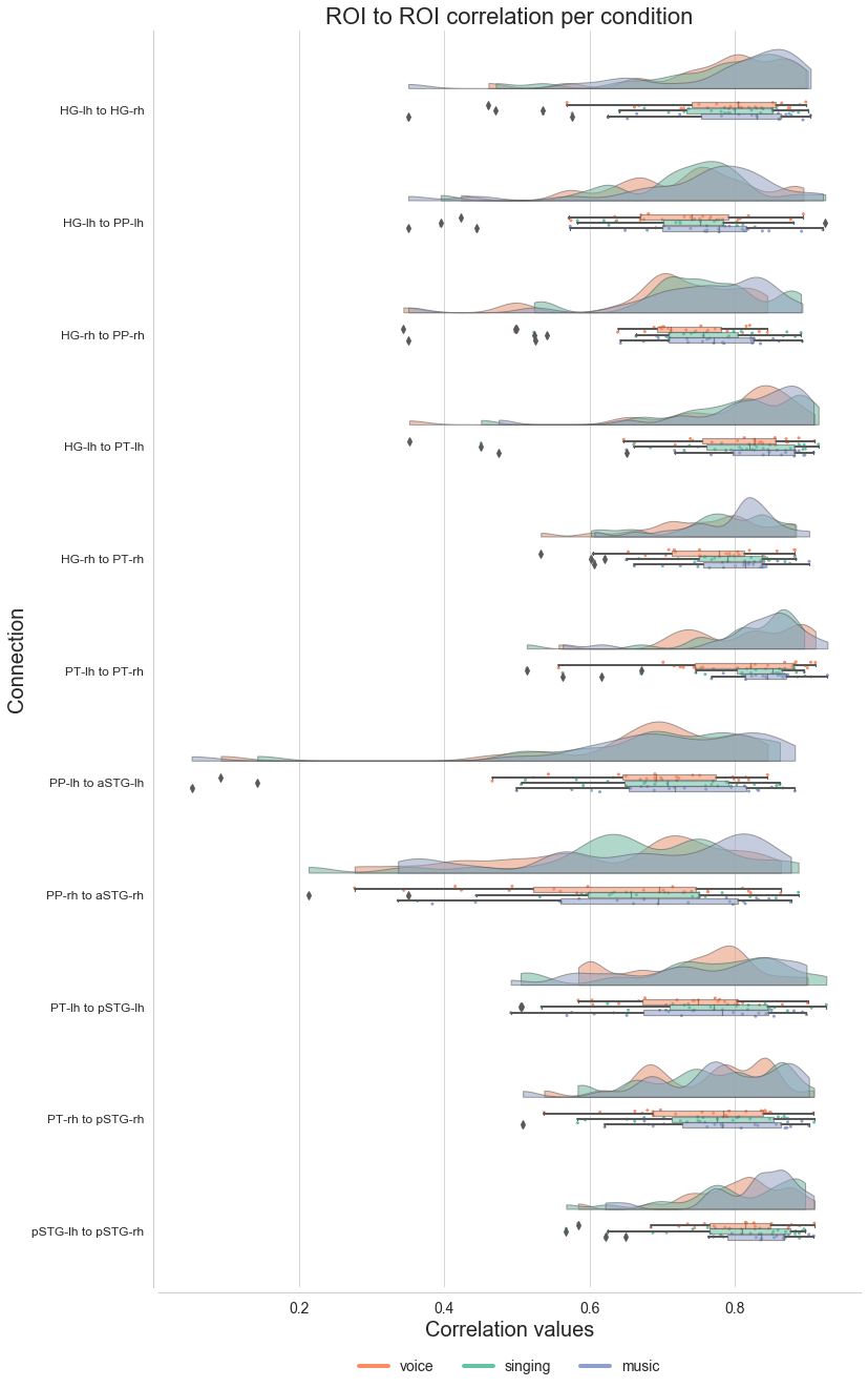
Now that we have computed the ROI to ROI correlation in our reduced auditory cortex network model for each participant and condition, as well as investigated the outputs on a descriptive level, it is time to compute some statistics. More precisely, we will assess two things: (1) which connections are significantly different from 0 for each condition and (2) which connections differ significantly between conditions.
Comparison of condition-specific functional connectivity
In order to assess which connections are significantly different from 0 for a given condition, we will compute a one-sample permutation test per connection and condition. This approach entails generating a null distribution via flipping the sign of a random number of values and recomputing the difference between the resulting mean and assumend 0 within each permutation fold. The original mean difference is then compared against this distribution and obtained p-values corrected for multiple comparisons through the Benjamin-Hochberg implementation of the FDR. To provide a detailed overview, we will do that step by step on an example, the voice condition. At first, we restrict our ROI to ROI DataFrame to include only data from the voice condition:
con_info_long_voice = con_info_long[con_info_long['condition']=='Voice']
con_info_long_voice
| part_cond | connection | cor_values | participant | condition | |
|---|---|---|---|---|---|
| 0 | sub-01_Voice | HG_lh_HG_rh | 0.729744 | sub-01 | Voice |
| 3 | sub-02_Voice | HG_lh_HG_rh | 0.830138 | sub-02 | Voice |
| 6 | sub-03_Voice | HG_lh_HG_rh | 0.875702 | sub-03 | Voice |
| 9 | sub-04_Voice | HG_lh_HG_rh | 0.661841 | sub-04 | Voice |
| 12 | sub-05_Voice | HG_lh_HG_rh | 0.897685 | sub-05 | Voice |
| 15 | sub-07_Voice | HG_lh_HG_rh | 0.805987 | sub-07 | Voice |
| 18 | sub-08_Voice | HG_lh_HG_rh | 0.791797 | sub-08 | Voice |
| 21 | sub-09_Voice | HG_lh_HG_rh | 0.873669 | sub-09 | Voice |
| 24 | sub-10_Voice | HG_lh_HG_rh | 0.819320 | sub-10 | Voice |
| 27 | sub-11_Voice | HG_lh_HG_rh | 0.889455 | sub-11 | Voice |
| 30 | sub-12_Voice | HG_lh_HG_rh | 0.793997 | sub-12 | Voice |
| 33 | sub-13_Voice | HG_lh_HG_rh | 0.750438 | sub-13 | Voice |
| 36 | sub-14_Voice | HG_lh_HG_rh | 0.774893 | sub-14 | Voice |
| 39 | sub-15_Voice | HG_lh_HG_rh | 0.725923 | sub-15 | Voice |
| 42 | sub-16_Voice | HG_lh_HG_rh | 0.804853 | sub-16 | Voice |
| 45 | sub-17_Voice | HG_lh_HG_rh | 0.852302 | sub-17 | Voice |
| 48 | sub-18_Voice | HG_lh_HG_rh | 0.864487 | sub-18 | Voice |
| 51 | sub-19_Voice | HG_lh_HG_rh | 0.762531 | sub-19 | Voice |
| 54 | sub-20_Voice | HG_lh_HG_rh | 0.809400 | sub-20 | Voice |
| 57 | sub-21_Voice | HG_lh_HG_rh | 0.461008 | sub-21 | Voice |
| 60 | sub-22_Voice | HG_lh_HG_rh | 0.858569 | sub-22 | Voice |
| 63 | sub-23_Voice | HG_lh_HG_rh | 0.667993 | sub-23 | Voice |
| 66 | sub-24_Voice | HG_lh_HG_rh | 0.569008 | sub-24 | Voice |
| 69 | sub-01_Voice | HG_lh_PP_lh | 0.730356 | sub-01 | Voice |
| 72 | sub-02_Voice | HG_lh_PP_lh | 0.877590 | sub-02 | Voice |
| 75 | sub-03_Voice | HG_lh_PP_lh | 0.739229 | sub-03 | Voice |
| 78 | sub-04_Voice | HG_lh_PP_lh | 0.669932 | sub-04 | Voice |
| 81 | sub-05_Voice | HG_lh_PP_lh | 0.807468 | sub-05 | Voice |
| 84 | sub-07_Voice | HG_lh_PP_lh | 0.574494 | sub-07 | Voice |
| 87 | sub-08_Voice | HG_lh_PP_lh | 0.766930 | sub-08 | Voice |
| ... | ... | ... | ... | ... | ... |
| 669 | sub-18_Voice | PT_rh_pSTG_rh | 0.841723 | sub-18 | Voice |
| 672 | sub-19_Voice | PT_rh_pSTG_rh | 0.843286 | sub-19 | Voice |
| 675 | sub-20_Voice | PT_rh_pSTG_rh | 0.718560 | sub-20 | Voice |
| 678 | sub-21_Voice | PT_rh_pSTG_rh | 0.697720 | sub-21 | Voice |
| 681 | sub-22_Voice | PT_rh_pSTG_rh | 0.784101 | sub-22 | Voice |
| 684 | sub-23_Voice | PT_rh_pSTG_rh | 0.687612 | sub-23 | Voice |
| 687 | sub-24_Voice | PT_rh_pSTG_rh | 0.537573 | sub-24 | Voice |
| 690 | sub-01_Voice | pSTG_lh_pSTG_rh | 0.771692 | sub-01 | Voice |
| 693 | sub-02_Voice | pSTG_lh_pSTG_rh | 0.814807 | sub-02 | Voice |
| 696 | sub-03_Voice | pSTG_lh_pSTG_rh | 0.827930 | sub-03 | Voice |
| 699 | sub-04_Voice | pSTG_lh_pSTG_rh | 0.735072 | sub-04 | Voice |
| 702 | sub-05_Voice | pSTG_lh_pSTG_rh | 0.889023 | sub-05 | Voice |
| 705 | sub-07_Voice | pSTG_lh_pSTG_rh | 0.744635 | sub-07 | Voice |
| 708 | sub-08_Voice | pSTG_lh_pSTG_rh | 0.826184 | sub-08 | Voice |
| 711 | sub-09_Voice | pSTG_lh_pSTG_rh | 0.792606 | sub-09 | Voice |
| 714 | sub-10_Voice | pSTG_lh_pSTG_rh | 0.584261 | sub-10 | Voice |
| 717 | sub-11_Voice | pSTG_lh_pSTG_rh | 0.909496 | sub-11 | Voice |
| 720 | sub-12_Voice | pSTG_lh_pSTG_rh | 0.846500 | sub-12 | Voice |
| 723 | sub-13_Voice | pSTG_lh_pSTG_rh | 0.758354 | sub-13 | Voice |
| 726 | sub-14_Voice | pSTG_lh_pSTG_rh | 0.874212 | sub-14 | Voice |
| 729 | sub-15_Voice | pSTG_lh_pSTG_rh | 0.816032 | sub-15 | Voice |
| 732 | sub-16_Voice | pSTG_lh_pSTG_rh | 0.873360 | sub-16 | Voice |
| 735 | sub-17_Voice | pSTG_lh_pSTG_rh | 0.850614 | sub-17 | Voice |
| 738 | sub-18_Voice | pSTG_lh_pSTG_rh | 0.792311 | sub-18 | Voice |
| 741 | sub-19_Voice | pSTG_lh_pSTG_rh | 0.877768 | sub-19 | Voice |
| 744 | sub-20_Voice | pSTG_lh_pSTG_rh | 0.827523 | sub-20 | Voice |
| 747 | sub-21_Voice | pSTG_lh_pSTG_rh | 0.723124 | sub-21 | Voice |
| 750 | sub-22_Voice | pSTG_lh_pSTG_rh | 0.786322 | sub-22 | Voice |
| 753 | sub-23_Voice | pSTG_lh_pSTG_rh | 0.808971 | sub-23 | Voice |
| 756 | sub-24_Voice | pSTG_lh_pSTG_rh | 0.684387 | sub-24 | Voice |
253 rows × 5 columns
Next, we will set up a small for-loop that computes the mean, mean difference and p value for each connection:
list_con = []
list_mean = []
list_mean_diff = []
list_p_values = []
for connection in con_info_long_voice['connection'].unique():
print('working on connection: %s' %connection)
list_con.append(connection)
df_tmp = con_info_long_voice[con_info_long_voice['connection']==connection]
list_mean.append(df_tmp['cor_values'].mean())
list_mean_diff.append(nnstats.permtest_1samp(df_tmp['cor_values'], 0.0)[0])
list_p_values.append(nnstats.permtest_1samp(df_tmp['cor_values'], 0.0)[1])
working on connection: HG_lh_HG_rh
working on connection: HG_lh_PP_lh
working on connection: HG_rh_PP_rh
working on connection: HG_lh_PT_lh
working on connection: HG_rh_PT_rh
working on connection: PT_lh_PT_rh
working on connection: PP_lh_aSTG_lh
working on connection: PP_rh_aSTG_rh
working on connection: PT_lh_pSTG_lh
working on connection: PT_rh_pSTG_rh
working on connection: pSTG_lh_pSTG_rh
As usual, we will pack everything into a DataFrame to make things easier:
con_info_long_voice_stats = pd.DataFrame({'connection': list_con, 'mean': list_mean, 'mean_diff': list_mean_diff, 'p_value': list_p_values})
con_info_long_voice_stats
| connection | mean | mean_diff | p_value | |
|---|---|---|---|---|
| 0 | HG_lh_HG_rh | 0.776989 | 0.776989 | 0.000999 |
| 1 | HG_lh_PP_lh | 0.723761 | 0.723761 | 0.000999 |
| 2 | HG_rh_PP_rh | 0.706425 | 0.706425 | 0.000999 |
| 3 | HG_lh_PT_lh | 0.791526 | 0.791526 | 0.000999 |
| 4 | HG_rh_PT_rh | 0.761162 | 0.761162 | 0.000999 |
| 5 | PT_lh_PT_rh | 0.805668 | 0.805668 | 0.000999 |
| 6 | PP_lh_aSTG_lh | 0.674060 | 0.674060 | 0.000999 |
| 7 | PP_rh_aSTG_rh | 0.631744 | 0.631744 | 0.000999 |
| 8 | PT_lh_pSTG_lh | 0.737993 | 0.737993 | 0.000999 |
| 9 | PT_rh_pSTG_rh | 0.757304 | 0.757304 | 0.000999 |
| 10 | pSTG_lh_pSTG_rh | 0.800660 | 0.800660 | 0.000999 |
So far, our p-values are not corrected for multiple comparisons and thus we use the great pingouin package to do that. All we need to do is provide the list of our uncorrected p-values and create a new column in our DataFrame to store the obtained corrected p-values.
con_info_long_voice_stats['p_values_FDR'] = multicomp(con_info_long_voice_stats['p_value'].to_list(), alpha=0.05, method='fdr_bh')[1]
con_info_long_voice_stats
| connection | mean | mean_diff | p_value | p_values_FDR | |
|---|---|---|---|---|---|
| 0 | HG_lh_HG_rh | 0.776989 | 0.776989 | 0.000999 | 0.000999 |
| 1 | HG_lh_PP_lh | 0.723761 | 0.723761 | 0.000999 | 0.000999 |
| 2 | HG_rh_PP_rh | 0.706425 | 0.706425 | 0.000999 | 0.000999 |
| 3 | HG_lh_PT_lh | 0.791526 | 0.791526 | 0.000999 | 0.000999 |
| 4 | HG_rh_PT_rh | 0.761162 | 0.761162 | 0.000999 | 0.000999 |
| 5 | PT_lh_PT_rh | 0.805668 | 0.805668 | 0.000999 | 0.000999 |
| 6 | PP_lh_aSTG_lh | 0.674060 | 0.674060 | 0.000999 | 0.000999 |
| 7 | PP_rh_aSTG_rh | 0.631744 | 0.631744 | 0.000999 | 0.000999 |
| 8 | PT_lh_pSTG_lh | 0.737993 | 0.737993 | 0.000999 | 0.000999 |
| 9 | PT_rh_pSTG_rh | 0.757304 | 0.757304 | 0.000999 | 0.000999 |
| 10 | pSTG_lh_pSTG_rh | 0.800660 | 0.800660 | 0.000999 | 0.000999 |
Coolio, now to visualization. While the DataFrame is nicely structured and informative, a corresponding graphic would be useful as well. What we are going to do is reusing steps from above and bring our DataFrame values back into the correlation matrix/network structure. Importantly, we will do that for mean values but only those which p-value are surviving thethreshold (p<=0.05).
voice_stats = np.zeros_like(network_structure_reduced)
voice_stats[connection_analyses_indices] = [row['mean'] if row['p_values_FDR'] <= 0.05 else np.nan for i, row in con_info_long_voice_stats.iterrows()]
voice_stats[voice_stats == 0] = np.nan
With that, we can plot the results as we did before:
fig = px.imshow(voice_stats, x=atlas_rois_df['regions'], y=atlas_rois_df['regions'],
color_continuous_scale='darkmint_r')
fig.update_layout(coloraxis_showscale=True)
fig['layout'].update(plot_bgcolor='white')
plot(fig, filename = 'ac_network_stats-voice.html')
display(HTML('ac_network_stats-voice.html'))
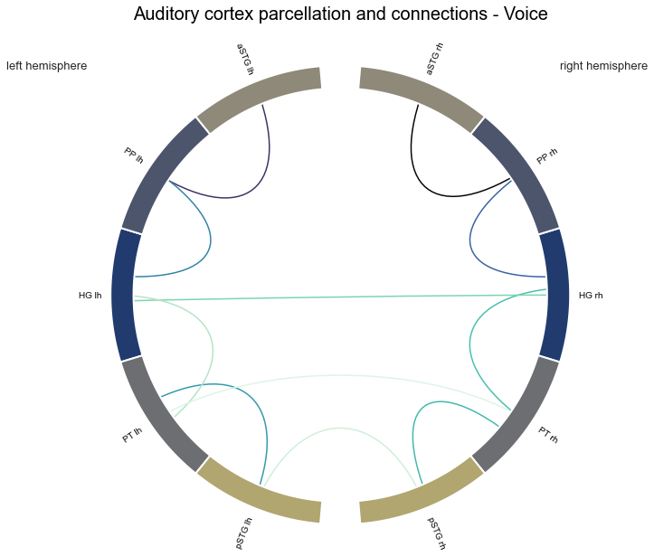
And the connectome version:
plot_auditory_cortex_connectome(voice_stats, atlas_info=atlas_rois_df, name='Voice', model=False)

Nice, some informative and easy to grasp figures to visualize the results of the statistical analyses. As we don’t want to run all this every time for each condition, we pack everything into a function. While doing so, we will also extend it a bit to support not only one-sample permutation tests for a single condition but also two sample related permutation tests for comparisons between conditions. The latter will be explained in more detail later:
def connection_stats(condition):
if len(condition) == 1:
print('Computing stats for condition: %s.' %condition[0])
plot_name = condition[0]
plot_name_graphic = condition[0]
else:
print('Computing stats for difference between %s and %s.' %(condition[0], condition[1]))
plot_name = '%s vs %s' %(condition[0], condition[1])
plot_name_graphic = '%svs%s' %(condition[0], condition[1])
con_info_long_tmp = con_info_long[con_info_long['condition'].isin(condition)]
list_con = []
list_mean = []
list_mean_2 = []
list_mean_diff = []
list_p_values = []
for connection in con_info_long_tmp['connection'].unique():
print('working on connection: %s' %connection)
list_con.append(connection)
df_tmp = con_info_long_tmp[con_info_long_tmp['connection']==connection]
if len(condition) == 1:
list_mean.append(df_tmp['cor_values'].mean())
list_mean_diff.append(nnstats.permtest_1samp(df_tmp['cor_values'], 0.0)[0])
list_p_values.append(nnstats.permtest_1samp(df_tmp['cor_values'], 0.0)[1])
con_info_long_tmp_stats = pd.DataFrame({'connection': list_con, 'mean': list_mean, 'mean_diff': list_mean_diff, 'p_value': list_p_values})
con_info_long_tmp_stats['p_values_FDR'] = multicomp(con_info_long_tmp_stats['p_value'].to_list(), alpha=0.05, method='fdr_bh')[1]
else:
list_mean.append(df_tmp[df_tmp['condition'] == condition[0]]['cor_values'].mean())
list_mean_2.append(df_tmp[df_tmp['condition'] == condition[1]]['cor_values'].mean())
list_mean_diff.append(nnstats.permtest_rel(df_tmp[df_tmp['condition'] == condition[0]]['cor_values'],
df_tmp[df_tmp['condition'] == condition[1]]['cor_values'])[0])
list_p_values.append(nnstats.permtest_rel(df_tmp[df_tmp['condition'] == condition[0]]['cor_values'],
df_tmp[df_tmp['condition'] == condition[1]]['cor_values'])[1])
con_info_long_tmp_stats = pd.DataFrame({'connection': list_con, 'mean_%s' %condition[0]: list_mean, 'mean_%s' %condition[1]: list_mean_2,
'mean_diff': list_mean_diff, 'p_value': list_p_values})
con_info_long_tmp_stats['p_values_FDR'] = multicomp(con_info_long_tmp_stats['p_value'].to_list(), alpha=0.05, method='fdr_bh')[1]
tmp_stats = np.zeros_like(network_structure_reduced)
tmp_stats[connection_analyses_indices] = [row['mean'] if row['p_values_FDR'] <= 0.05 else np.nan for i, row in con_info_long_tmp_stats.iterrows()]
tmp_stats[tmp_stats == 0] = np.nan
if np.isnan(tmp_stats).all():
print('No connection significant.')
else:
fig = px.imshow(tmp_stats, x=atlas_rois_df['regions'], y=atlas_rois_df['regions'],
color_continuous_scale='darkmint_r')
fig.update_layout(coloraxis_showscale=True, font_family="Arial")
fig.update_layout(title={'text': 'Connection statistics (mean, FDR<=0.05) - %s' %plot_name, 'y':0.9, 'x':0.5, 'xanchor': 'center', 'yanchor': 'top'})
fig['layout'].update(plot_bgcolor='white')
plot(fig, filename = 'ac_network_stats-%s.html' %plot_name_graphic)
display(HTML('ac_network_stats-%s.html' %plot_name_graphic))
plot_auditory_cortex_connectome(tmp_stats, atlas_info=atlas_rois_df, name=plot_name, model=False)
return con_info_long_tmp_stats, tmp_stats
To be sure everything works as expected, let’s recompute the outputs for the voice condition:
con_voice, stats_voice = connection_stats(['Voice'])
Computing stats for condition: Voice.
working on connection: HG_lh_HG_rh
working on connection: HG_lh_PP_lh
working on connection: HG_rh_PP_rh
working on connection: HG_lh_PT_lh
working on connection: HG_rh_PT_rh
working on connection: PT_lh_PT_rh
working on connection: PP_lh_aSTG_lh
working on connection: PP_rh_aSTG_rh
working on connection: PT_lh_pSTG_lh
working on connection: PT_rh_pSTG_rh
working on connection: pSTG_lh_pSTG_rh
That looks about right. Now, we can easily apply the function to compute the statistics for the other conditions. At first, singing:
con_singing, stats_singing = connection_stats(['Singing'])
Computing stats for condition: Singing.
working on connection: HG_lh_HG_rh
working on connection: HG_lh_PP_lh
working on connection: HG_rh_PP_rh
working on connection: HG_lh_PT_lh
working on connection: HG_rh_PT_rh
working on connection: PT_lh_PT_rh
working on connection: PP_lh_aSTG_lh
working on connection: PP_rh_aSTG_rh
working on connection: PT_lh_pSTG_lh
working on connection: PT_rh_pSTG_rh
working on connection: pSTG_lh_pSTG_rh

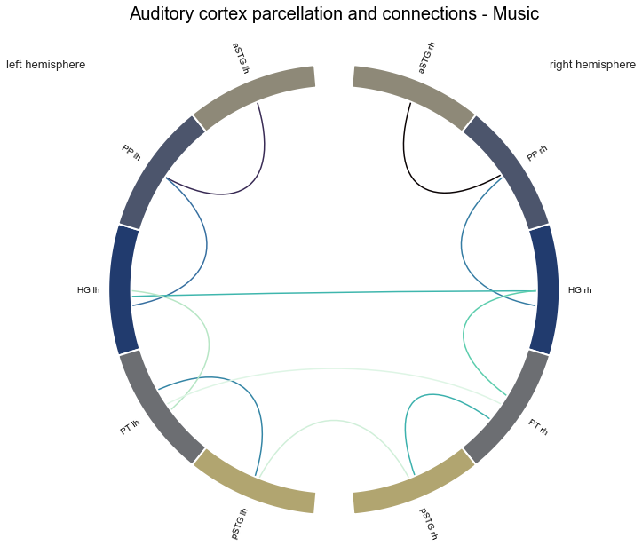
And second, music:
con_music, stats_music = connection_stats(['Music'])
Computing stats for condition: Music.
working on connection: HG_lh_HG_rh
working on connection: HG_lh_PP_lh
working on connection: HG_rh_PP_rh
working on connection: HG_lh_PT_lh
working on connection: HG_rh_PT_rh
working on connection: PT_lh_PT_rh
working on connection: PP_lh_aSTG_lh
working on connection: PP_rh_aSTG_rh
working on connection: PT_lh_pSTG_lh
working on connection: PT_rh_pSTG_rh
working on connection: pSTG_lh_pSTG_rh
After computing the statistics for a single condition via one sample permutation tests, it is time to compare connections between conditions via two sample permutation tests. Here, null distributions are generated by exchanging a random number of values between conditions and recomputing the difference in means within a given permutation fold. The original difference in means is then compared to the obtained distribution. Using our function, all we need to do to achieve this is providing a list of the two conditions we want to compare. Everything else works as before. Let’s start with the comparison between the voice and singing condition.
con_voice_singing, stats_voice_singing = connection_stats(['Voice', 'Singing'])
Computing stats for difference between Voice and Singing.
working on connection: HG_lh_HG_rh
working on connection: HG_lh_PP_lh
working on connection: HG_rh_PP_rh
working on connection: HG_lh_PT_lh
working on connection: HG_rh_PT_rh
working on connection: PT_lh_PT_rh
working on connection: PP_lh_aSTG_lh
working on connection: PP_rh_aSTG_rh
working on connection: PT_lh_pSTG_lh
working on connection: PT_rh_pSTG_rh
working on connection: pSTG_lh_pSTG_rh
No connection significant.
We do not see any graphics, because no connection is significantly different between the conditions as indicated by the output. How do things look for the comparison between voice and music?
con_voice_music, stats_voice_music = connection_stats(['Voice', 'Music'])
Computing stats for difference between Voice and Music.
working on connection: HG_lh_HG_rh
working on connection: HG_lh_PP_lh
working on connection: HG_rh_PP_rh
working on connection: HG_lh_PT_lh
working on connection: HG_rh_PT_rh
working on connection: PT_lh_PT_rh
working on connection: PP_lh_aSTG_lh
working on connection: PP_rh_aSTG_rh
working on connection: PT_lh_pSTG_lh
working on connection: PT_rh_pSTG_rh
working on connection: pSTG_lh_pSTG_rh
No connection significant.
The same, no connection is significantly different. Last but not least: the comparison between music and singing:
con_music_singing, stats_music_singing = connection_stats(['Music', 'Singing'])
Computing stats for difference between Music and Singing.
working on connection: HG_lh_HG_rh
working on connection: HG_lh_PP_lh
working on connection: HG_rh_PP_rh
working on connection: HG_lh_PT_lh
working on connection: HG_rh_PT_rh
working on connection: PT_lh_PT_rh
working on connection: PP_lh_aSTG_lh
working on connection: PP_rh_aSTG_rh
working on connection: PT_lh_pSTG_lh
working on connection: PT_rh_pSTG_rh
working on connection: pSTG_lh_pSTG_rh
No connection significant.
Same same. This comparison also concludes the ROI to ROI correlation analyses of the the Connectivity analyses.