Meta-analysis
Within this section the meta-analyses, that is ROI co-activation and meta-analyses - searchlight/gradient map comparison, are shown, explained and set up in a way that they can be rerun and reproduced. In short, we employed the Neurosynth database to assess ROI co-activation patterns and Neuroquery to obtain condition-specific meta-analytic maps. The latter were compared to the searchlight and gradient maps computed in the previous steps, via a combination of spatial null models and permutation correlation analyses as implemented in the BrainSmash toolbox. These analyses were conducted to investigate if meta-analyses based on large-scale datasets support aspects of the functional profiles and if the obtained results are generalizable to a certain extent. The analysis was divided into the following sections:
Prerequisites
Auditory cortex ROIs
ROI co-activation
Neurosynth database
Co-activation analyses
Condition-specific meta-analytic maps
Meta-analytic map - searchlight/gradient map comparison
Spatial null models
Permutation correlation analyses
We provide more detailed information and explanations in the respective sections. As mentioned before, we’re working with derivatives here and thus we can share them, meaning that you can rerun the analyses either by downloading this page as a Jupyter Notebook (via the download button at the top) or interactively via a cloud instance through the amazing mybinder project (the little rocket at the top). We recommend the later to spare installation and conda environment related problems. One more thing… Please note, that here derivatives refers to the computed permuted meta-analytic maps (i.e. (spatial null models)) which we provide via the project’s OSF page because their computation is computationally very expensive and would never run via the resources available through binder. However, we included the code and explanations depicting how this steps were run. The code that will download the required data is included in the respective sections.
As usual, we will start with importing all necessary modules and functions.
from os.path import join as opj
from os.path import basename as opb
from nilearn.plotting import plot_img, plot_anat, plot_surf_stat_map, view_img_on_surf, plot_matrix
from nilearn.image import resample_to_img, math_img, load_img
from nilearn.input_data import NiftiMasker
from nilearn import datasets
from nilearn.surface import vol_to_surf
import nibabel as nb
import numpy as np
import pandas as pd
import matplotlib.pyplot as plt
import seaborn as sns
import plotly
import plotly.graph_objects as go
from IPython.core.display import display, HTML
from plotly.offline import init_notebook_mode, plot
from neurosynth import Dataset
from neurosynth import decode, network
from neurosynth.base import dataset
from neuroquery import fetch_neuroquery_model, NeuroQueryModel
from matplotlib.patches import Arc
from glob import glob
from matplotlib import colors
from matplotlib.lines import Line2D
from scipy.spatial.distance import squareform, pdist
from scipy import stats
from brainsmash.mapgen.base import Base
from brainsmash.mapgen.sampled import Sampled
from brainsmash.mapgen.eval import sampled_fit
from brainsmash.mapgen.memmap import txt2memmap
from brainsmash.mapgen.stats import pearsonr, nonparp
Let’s also gather and set some important paths. This includes the path to the general derivatives directory, as well as analyses specific ones. In more detail, we of course aim to keep it as BIDS-y as possible and therefore set a path for the meta-analyses here. To keep results and necessary prerequisites separate (keeping it tidy), we also create a dedicated directory which will include the neurosynth database and specify where the results from the previous steps are.
meta_dir = '/data/mvs/derivatives/meta_analyses'
roi_mask_path ='/data/mvs/derivatives/ROIs_masks/'
prereq_path = '/data/mvs/derivatives/meta_analyses/prerequisites/'
results_path = '/data/mvs/derivatives/meta_analyses/results'
sl_dir = '/data/mvs/derivatives/MVPA/results/searchlight/'
grad_dir = '/data/mvs/derivatives/connectivity/results/voxel_to_voxel/'
Prerequisites
Auditory Cortex ROIs
At first, we need to gather our auditory cortex ROIs that we used throughout the previous analyses, as they are required for the ROI co-activation analyses. Just as a reminder, this includes the STP, including HG, PP and PT, and the upper banks of the STG, including aSTG and pSTG. At first, we gather them within a list (please note that we will exclude the auditory cortex masks):
rois = [roi for roi in glob(opj(roi_mask_path, '*.nii.gz'))
if not 'AC' in opb(roi)]
rois.sort()
rois
['/data/mvs/derivatives/ROIs_masks/tpl-MNI152NLin6Sym_res_02_desc-HGleft_mask.nii.gz',
'/data/mvs/derivatives/ROIs_masks/tpl-MNI152NLin6Sym_res_02_desc-HGright_mask.nii.gz',
'/data/mvs/derivatives/ROIs_masks/tpl-MNI152NLin6Sym_res_02_desc-PPleft_mask.nii.gz',
'/data/mvs/derivatives/ROIs_masks/tpl-MNI152NLin6Sym_res_02_desc-PPright_mask.nii.gz',
'/data/mvs/derivatives/ROIs_masks/tpl-MNI152NLin6Sym_res_02_desc-PTleft_mask.nii.gz',
'/data/mvs/derivatives/ROIs_masks/tpl-MNI152NLin6Sym_res_02_desc-PTright_mask.nii.gz',
'/data/mvs/derivatives/ROIs_masks/tpl-MNI152NLin6Sym_res_02_desc-aSTGleft_mask.nii.gz',
'/data/mvs/derivatives/ROIs_masks/tpl-MNI152NLin6Sym_res_02_desc-aSTGright_mask.nii.gz',
'/data/mvs/derivatives/ROIs_masks/tpl-MNI152NLin6Sym_res_02_desc-pSTGleft_mask.nii.gz',
'/data/mvs/derivatives/ROIs_masks/tpl-MNI152NLin6Sym_res_02_desc-pSTGright_mask.nii.gz']
Let’s pack the paths and the ROI names in lists to ease up later processing steps:
HG_left = rois[0]
HG_right = rois[1]
PP_left = rois[2]
PP_right = rois[3]
PT_left = rois[4]
PT_right = rois[5]
aSTG_left = rois[6]
aSTG_right = rois[7]
pSTG_left = rois[8]
pSTG_right = rois[9]
list_rois = [HG_left, HG_right, PP_left, PP_right, PT_left, PT_right, aSTG_left, aSTG_right, pSTG_left, pSTG_right]
list_rois_names = ['HG_left', 'HG_right', 'PP_left', 'PP_right', 'PT_left', 'PT_right',
'aSTG_left', 'aSTG_right', 'pSTG_left', 'pSTG_right']
We will need the auditory cortex mask later on as well, thus let’s set it:
ac_mask = opj(roi_mask_path, 'tpl-MNI152NLin6Sym_res_02_desc-AC_mask.nii.gz')
So far so good. As it has been a while since we last saw them, let’s have a look by overlaying them on the MNI152 template brain:
#suppress contour related warnings
import warnings
warnings.filterwarnings("ignore")
sns.set_style('white')
plt.rcParams["font.family"] = "Arial"
fig=plt.figure(num=None, figsize=(12, 6))
check_ROIs = plot_anat(cut_coords=[-55, -34, 7], figure=fig, draw_cross=False)
check_ROIs.add_contours(HG_left,
colors=[sns.color_palette('cividis', 5)[0]],
filled=True)
check_ROIs.add_contours(PP_left,
colors=[sns.color_palette('cividis', 5)[1]],
filled=True)
check_ROIs.add_contours(PT_left,
colors=[sns.color_palette('cividis', 5)[2]],
filled=True)
check_ROIs.add_contours(aSTG_left,
colors=[sns.color_palette('cividis', 5)[3]],
filled=True)
check_ROIs.add_contours(pSTG_left,
colors=[sns.color_palette('cividis', 5)[4]],
filled=True)
check_ROIs.add_contours(HG_right,
colors=[sns.color_palette('cividis', 5)[0]],
filled=True)
check_ROIs.add_contours(PP_right,
colors=[sns.color_palette('cividis', 5)[1]],
filled=True)
check_ROIs.add_contours(PT_right,
colors=[sns.color_palette('cividis', 5)[2]],
filled=True)
check_ROIs.add_contours(aSTG_right,
colors=[sns.color_palette('cividis', 5)[3]],
filled=True)
check_ROIs.add_contours(pSTG_right,
colors=[sns.color_palette('cividis', 5)[4]],
filled=True)
check_ROIs.add_contours(ac_mask,
levels=[0], colors='black')
mask_legend = [Line2D([0], [0], color='black', lw=4, label='Auditory Cortex\n mask', alpha=0.8)]
first_legend = plt.legend(handles=mask_legend, bbox_to_anchor=(1.5,0.3), loc='right')
plt.gca().add_artist(first_legend)
roi_legend = [Line2D([0], [0], color=sns.color_palette('cividis', 5)[3], lw=4, label='aSTg'),
Line2D([0], [0], color=sns.color_palette('cividis', 5)[1], lw=4, label='PP'),
Line2D([0], [0], color=sns.color_palette('cividis', 5)[0], lw=4, label='HG'),
Line2D([0], [0], color=sns.color_palette('cividis', 5)[2], lw=4, label='PT'),
Line2D([0], [0], color=sns.color_palette('cividis', 5)[4], lw=4, label='pSTG')]
plt.legend(handles=roi_legend, bbox_to_anchor=(1.5,0.5), loc="right", title='ROIs')
plt.text(-215, 90, 'Auditory cortex ROIs',
fontsize=22)
Text(-215, 90, 'Auditory cortex ROIs')
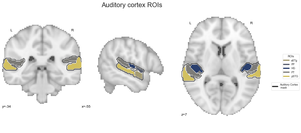
That looks about right and we already have everything we need to start with our analyses, starting with the ROI co-activation.
ROI co-activation
In this first set of meta-analyses we will investigate the so-called co-activation pattern of our ROIs. In more detail, we will use the latest version of the Neurosynth database to perform meta-analytic contrasts to evaluate which voxels have a high probability of being co-activated with a given ROI. The resulting maps will thus show us which voxels/regions are likely being active when there is activation in a given ROI. To achieve this we basically only need two steps: getting the neurosynth database and running the co-activation analyses.
Neurosynth database
The Neurosynth database is a large-scale repository targeted for meta-analyses, containing thousands of peak activations across the entire range of neuroscientific literature. Here, we utilize the latest version, v0.7 including over 14k studies. As everything is open and build around a great API, we can easily download the neurosynth files:
ns_data_dir = opj(prereq_path, 'neurosynth_data/')
dataset.download(ns_data_dir, unpack=True)
Downloading the latest Neurosynth files: https://github.com/neurosynth/neurosynth-data/blob/master/current_data.tar.gz?raw=true bytes: 1
8192 [819200.00%16384 [1638400.00%24576 [2457600.00%32768 [3276800.00%40960 [4096000.00%49152 [4915200.00%57344 [5734400.00%65536 [6553600.00%73728 [7372800.00%81920 [8192000.00%90112 [9011200.00%98304 [9830400.00%106496 [10649600.00%114688 [11468800.00%122880 [12288000.00%131072 [13107200.00%139264 [13926400.00%147456 [14745600.00%155648 [15564800.00%163840 [16384000.00%172032 [17203200.00%180224 [18022400.00%188416 [18841600.00%196608 [19660800.00%204800 [20480000.00%212992 [21299200.00%221184 [22118400.00%229376 [22937600.00%237568 [23756800.00%245760 [24576000.00%253952 [25395200.00%262144 [26214400.00%270336 [27033600.00%278528 [27852800.00%286720 [28672000.00%294912 [29491200.00%303104 [30310400.00%311296 [31129600.00%319488 [31948800.00%327680 [32768000.00%335872 [33587200.00%344064 [34406400.00%352256 [35225600.00%360448 [36044800.00%368640 [36864000.00%376832 [37683200.00%385024 [38502400.00%393216 [39321600.00%401408 [40140800.00%409600 [40960000.00%417792 [41779200.00%425984 [42598400.00%434176 [43417600.00%442368 [44236800.00%450560 [45056000.00%458752 [45875200.00%466944 [46694400.00%475136 [47513600.00%483328 [48332800.00%491520 [49152000.00%499712 [49971200.00%507904 [50790400.00%516096 [51609600.00%524288 [52428800.00%532480 [53248000.00%540672 [54067200.00%548864 [54886400.00%557056 [55705600.00%565248 [56524800.00%573440 [57344000.00%581632 [58163200.00%589824 [58982400.00%598016 [59801600.00%606208 [60620800.00%614400 [61440000.00%622592 [62259200.00%630784 [63078400.00%638976 [63897600.00%647168 [64716800.00%655360 [65536000.00%663552 [66355200.00%671744 [67174400.00%679936 [67993600.00%688128 [68812800.00%696320 [69632000.00%704512 [70451200.00%712704 [71270400.00%720896 [72089600.00%729088 [72908800.00%737280 [73728000.00%745472 [74547200.00%753664 [75366400.00%761856 [76185600.00%770048 [77004800.00%778240 [77824000.00%786432 [78643200.00%794624 [79462400.00%802816 [80281600.00%811008 [81100800.00%819200 [81920000.00%827392 [82739200.00%835584 [83558400.00%843776 [84377600.00%851968 [85196800.00%860160 [86016000.00%868352 [86835200.00%876544 [87654400.00%884736 [88473600.00%892928 [89292800.00%901120 [90112000.00%909312 [90931200.00%917504 [91750400.00%925696 [92569600.00%933888 [93388800.00%942080 [94208000.00%950272 [95027200.00%958464 [95846400.00%966656 [96665600.00%974848 [97484800.00%983040 [98304000.00%991232 [99123200.00%999424 [99942400.00%1007616 [100761600.00%1015808 [101580800.00%1024000 [102400000.00%1032192 [103219200.00%1040384 [104038400.00%1048576 [104857600.00%1056768 [105676800.00%1064960 [106496000.00%1073152 [107315200.00%1081344 [108134400.00%1089536 [108953600.00%1097728 [109772800.00%1105920 [110592000.00%1114112 [111411200.00%1122304 [112230400.00%1130496 [113049600.00%1138688 [113868800.00%1146880 [114688000.00%1155072 [115507200.00%1163264 [116326400.00%1171456 [117145600.00%1179648 [117964800.00%1187840 [118784000.00%1196032 [119603200.00%1204224 [120422400.00%1212416 [121241600.00%1220608 [122060800.00%1228800 [122880000.00%1236992 [123699200.00%1245184 [124518400.00%1253376 [125337600.00%1261568 [126156800.00%1269760 [126976000.00%1277952 [127795200.00%1286144 [128614400.00%1294336 [129433600.00%1302528 [130252800.00%1310720 [131072000.00%1318912 [131891200.00%1327104 [132710400.00%1335296 [133529600.00%1343488 [134348800.00%1351680 [135168000.00%1359872 [135987200.00%1368064 [136806400.00%1376256 [137625600.00%1384448 [138444800.00%1392640 [139264000.00%1400832 [140083200.00%1409024 [140902400.00%1417216 [141721600.00%1425408 [142540800.00%1433600 [143360000.00%1441792 [144179200.00%1449984 [144998400.00%1458176 [145817600.00%1466368 [146636800.00%1474560 [147456000.00%1482752 [148275200.00%1490944 [149094400.00%1499136 [149913600.00%1507328 [150732800.00%1515520 [151552000.00%1523712 [152371200.00%1531904 [153190400.00%1540096 [154009600.00%1548288 [154828800.00%1556480 [155648000.00%1564672 [156467200.00%1572864 [157286400.00%1581056 [158105600.00%1589248 [158924800.00%1597440 [159744000.00%1605632 [160563200.00%1613824 [161382400.00%1622016 [162201600.00%1630208 [163020800.00%1638400 [163840000.00%1646592 [164659200.00%1654784 [165478400.00%1662976 [166297600.00%1671168 [167116800.00%1679360 [167936000.00%1687552 [168755200.00%1695744 [169574400.00%1703936 [170393600.00%1712128 [171212800.00%1720320 [172032000.00%1728512 [172851200.00%1736704 [173670400.00%1744896 [174489600.00%1753088 [175308800.00%1761280 [176128000.00%1769472 [176947200.00%1777664 [177766400.00%1785856 [178585600.00%1794048 [179404800.00%1802240 [180224000.00%1810432 [181043200.00%1818624 [181862400.00%1826816 [182681600.00%1835008 [183500800.00%1843200 [184320000.00%1851392 [185139200.00%1859584 [185958400.00%1867776 [186777600.00%1875968 [187596800.00%1884160 [188416000.00%1892352 [189235200.00%1900544 [190054400.00%1908736 [190873600.00%1916928 [191692800.00%1925120 [192512000.00%1933312 [193331200.00%1941504 [194150400.00%1949696 [194969600.00%1957888 [195788800.00%1966080 [196608000.00%1974272 [197427200.00%1982464 [198246400.00%1990656 [199065600.00%1998848 [199884800.00%2007040 [200704000.00%2015232 [201523200.00%2023424 [202342400.00%2031616 [203161600.00%2039808 [203980800.00%2048000 [204800000.00%2056192 [205619200.00%2064384 [206438400.00%2072576 [207257600.00%2080768 [208076800.00%2088960 [208896000.00%2097152 [209715200.00%2105344 [210534400.00%2113536 [211353600.00%2121728 [212172800.00%2129920 [212992000.00%2138112 [213811200.00%2146304 [214630400.00%2154496 [215449600.00%2162688 [216268800.00%2170880 [217088000.00%2179072 [217907200.00%2187264 [218726400.00%2195456 [219545600.00%2203648 [220364800.00%2211840 [221184000.00%2220032 [222003200.00%2228224 [222822400.00%2236416 [223641600.00%2244608 [224460800.00%2252800 [225280000.00%2260992 [226099200.00%2269184 [226918400.00%2277376 [227737600.00%2285568 [228556800.00%2293760 [229376000.00%2301952 [230195200.00%2310144 [231014400.00%2318336 [231833600.00%2326528 [232652800.00%2334720 [233472000.00%2342912 [234291200.00%2351104 [235110400.00%2359296 [235929600.00%2367488 [236748800.00%2375680 [237568000.00%2383872 [238387200.00%2392064 [239206400.00%2400256 [240025600.00%2408448 [240844800.00%2416640 [241664000.00%2424832 [242483200.00%2433024 [243302400.00%2441216 [244121600.00%2449408 [244940800.00%2457600 [245760000.00%2465792 [246579200.00%2473984 [247398400.00%2482176 [248217600.00%2490368 [249036800.00%2498560 [249856000.00%2506752 [250675200.00%2514944 [251494400.00%2523136 [252313600.00%2531328 [253132800.00%2539520 [253952000.00%2547712 [254771200.00%2555904 [255590400.00%2564096 [256409600.00%2572288 [257228800.00%2580480 [258048000.00%2588672 [258867200.00%2596864 [259686400.00%2605056 [260505600.00%2613248 [261324800.00%2621440 [262144000.00%2629632 [262963200.00%2637824 [263782400.00%2646016 [264601600.00%2654208 [265420800.00%2662400 [266240000.00%2670592 [267059200.00%2678784 [267878400.00%2686976 [268697600.00%2695168 [269516800.00%2703360 [270336000.00%2711552 [271155200.00%2719744 [271974400.00%2727936 [272793600.00%2736128 [273612800.00%2744320 [274432000.00%2752512 [275251200.00%2760704 [276070400.00%2768896 [276889600.00%2777088 [277708800.00%2785280 [278528000.00%2793472 [279347200.00%2801664 [280166400.00%2809856 [280985600.00%2818048 [281804800.00%2826240 [282624000.00%2834432 [283443200.00%2842624 [284262400.00%2850816 [285081600.00%2859008 [285900800.00%2867200 [286720000.00%2875392 [287539200.00%2883584 [288358400.00%2891776 [289177600.00%2899968 [289996800.00%2908160 [290816000.00%2916352 [291635200.00%2924544 [292454400.00%2932736 [293273600.00%2940928 [294092800.00%2949120 [294912000.00%2957312 [295731200.00%2965504 [296550400.00%2973696 [297369600.00%2981888 [298188800.00%2990080 [299008000.00%2998272 [299827200.00%3006464 [300646400.00%3014656 [301465600.00%3022848 [302284800.00%3031040 [303104000.00%3039232 [303923200.00%3047424 [304742400.00%3055616 [305561600.00%3063808 [306380800.00%3072000 [307200000.00%3080192 [308019200.00%3088384 [308838400.00%3096576 [309657600.00%3104768 [310476800.00%3112960 [311296000.00%3121152 [312115200.00%3129344 [312934400.00%3137536 [313753600.00%3145728 [314572800.00%3153920 [315392000.00%3162112 [316211200.00%3170304 [317030400.00%3178496 [317849600.00%3186688 [318668800.00%3194880 [319488000.00%3203072 [320307200.00%3211264 [321126400.00%3219456 [321945600.00%3227648 [322764800.00%3235840 [323584000.00%3244032 [324403200.00%3252224 [325222400.00%3260416 [326041600.00%3268608 [326860800.00%3276800 [327680000.00%3284992 [328499200.00%3293184 [329318400.00%3301376 [330137600.00%3309568 [330956800.00%3317760 [331776000.00%3325952 [332595200.00%3334144 [333414400.00%3342336 [334233600.00%3350528 [335052800.00%3358720 [335872000.00%3366912 [336691200.00%3375104 [337510400.00%3383296 [338329600.00%3391488 [339148800.00%3399680 [339968000.00%3407872 [340787200.00%3416064 [341606400.00%3424256 [342425600.00%3432448 [343244800.00%3440640 [344064000.00%3448832 [344883200.00%3457024 [345702400.00%3465216 [346521600.00%3473408 [347340800.00%3481600 [348160000.00%3489792 [348979200.00%3497984 [349798400.00%3506176 [350617600.00%3514368 [351436800.00%3522560 [352256000.00%3530752 [353075200.00%3538944 [353894400.00%3547136 [354713600.00%3555328 [355532800.00%3563520 [356352000.00%3571712 [357171200.00%3579904 [357990400.00%3588096 [358809600.00%3596288 [359628800.00%3604480 [360448000.00%3612672 [361267200.00%3620864 [362086400.00%3629056 [362905600.00%3637248 [363724800.00%3645440 [364544000.00%3653632 [365363200.00%3661824 [366182400.00%3670016 [367001600.00%3678208 [367820800.00%3686400 [368640000.00%3694592 [369459200.00%3702784 [370278400.00%3710976 [371097600.00%3719168 [371916800.00%3727360 [372736000.00%3735552 [373555200.00%3743744 [374374400.00%3751936 [375193600.00%3760128 [376012800.00%3768320 [376832000.00%3776512 [377651200.00%3784704 [378470400.00%3792896 [379289600.00%3801088 [380108800.00%3809280 [380928000.00%3817472 [381747200.00%3825664 [382566400.00%3833856 [383385600.00%3842048 [384204800.00%3850240 [385024000.00%3858432 [385843200.00%3866624 [386662400.00%3874816 [387481600.00%3883008 [388300800.00%3891200 [389120000.00%3899392 [389939200.00%3907584 [390758400.00%3915776 [391577600.00%3923968 [392396800.00%3932160 [393216000.00%3940352 [394035200.00%3948544 [394854400.00%3956736 [395673600.00%3964928 [396492800.00%3973120 [397312000.00%3981312 [398131200.00%3989504 [398950400.00%3997696 [399769600.00%4005888 [400588800.00%4014080 [401408000.00%4022272 [402227200.00%4030464 [403046400.00%4038656 [403865600.00%4046848 [404684800.00%4055040 [405504000.00%4063232 [406323200.00%4071424 [407142400.00%4079616 [407961600.00%4087808 [408780800.00%4096000 [409600000.00%4104192 [410419200.00%4112384 [411238400.00%4120576 [412057600.00%4128768 [412876800.00%4136960 [413696000.00%4145152 [414515200.00%4153344 [415334400.00%4161536 [416153600.00%4169728 [416972800.00%4177920 [417792000.00%4186112 [418611200.00%4194304 [419430400.00%4202496 [420249600.00%4210688 [421068800.00%4218880 [421888000.00%4227072 [422707200.00%4235264 [423526400.00%4243456 [424345600.00%4251648 [425164800.00%4259840 [425984000.00%4268032 [426803200.00%4276224 [427622400.00%4284416 [428441600.00%4292608 [429260800.00%4300800 [430080000.00%4308992 [430899200.00%4317184 [431718400.00%4325376 [432537600.00%4333568 [433356800.00%4341760 [434176000.00%4349952 [434995200.00%4358144 [435814400.00%4366336 [436633600.00%4374528 [437452800.00%4382720 [438272000.00%4390912 [439091200.00%4399104 [439910400.00%4407296 [440729600.00%4415488 [441548800.00%4423680 [442368000.00%4431872 [443187200.00%4440064 [444006400.00%4448256 [444825600.00%4456448 [445644800.00%4464640 [446464000.00%4472832 [447283200.00%4481024 [448102400.00%4489216 [448921600.00%4497408 [449740800.00%4505600 [450560000.00%4513792 [451379200.00%4521984 [452198400.00%4530176 [453017600.00%4538368 [453836800.00%4546560 [454656000.00%4554752 [455475200.00%4562944 [456294400.00%4571136 [457113600.00%4579328 [457932800.00%4587520 [458752000.00%4595712 [459571200.00%4603904 [460390400.00%4612096 [461209600.00%4620288 [462028800.00%4628480 [462848000.00%4636672 [463667200.00%4644864 [464486400.00%4653056 [465305600.00%4661248 [466124800.00%4669440 [466944000.00%4677632 [467763200.00%4685824 [468582400.00%4694016 [469401600.00%4702208 [470220800.00%4710400 [471040000.00%4718592 [471859200.00%4726784 [472678400.00%4734976 [473497600.00%4743168 [474316800.00%4751360 [475136000.00%4759552 [475955200.00%4767744 [476774400.00%4775936 [477593600.00%4784128 [478412800.00%4792320 [479232000.00%4800512 [480051200.00%4808704 [480870400.00%4816896 [481689600.00%4825088 [482508800.00%4833280 [483328000.00%4841472 [484147200.00%4849664 [484966400.00%4857856 [485785600.00%4866048 [486604800.00%4874240 [487424000.00%4882432 [488243200.00%4890624 [489062400.00%4898816 [489881600.00%4907008 [490700800.00%4915200 [491520000.00%4923392 [492339200.00%4931584 [493158400.00%4939776 [493977600.00%4947968 [494796800.00%4956160 [495616000.00%4964352 [496435200.00%4972544 [497254400.00%4980736 [498073600.00%4988928 [498892800.00%4997120 [499712000.00%5005312 [500531200.00%5013504 [501350400.00%5021696 [502169600.00%5029888 [502988800.00%5038080 [503808000.00%5046272 [504627200.00%5054464 [505446400.00%5062656 [506265600.00%5070848 [507084800.00%5079040 [507904000.00%5087232 [508723200.00%5095424 [509542400.00%5103616 [510361600.00%5111808 [511180800.00%5120000 [512000000.00%5128192 [512819200.00%5136384 [513638400.00%5144576 [514457600.00%5152768 [515276800.00%5160960 [516096000.00%5169152 [516915200.00%5177344 [517734400.00%5185536 [518553600.00%5193728 [519372800.00%5201920 [520192000.00%5210112 [521011200.00%5218304 [521830400.00%5226496 [522649600.00%5234688 [523468800.00%5242880 [524288000.00%5251072 [525107200.00%5259264 [525926400.00%5267456 [526745600.00%5275648 [527564800.00%5283840 [528384000.00%5292032 [529203200.00%5300224 [530022400.00%5308416 [530841600.00%5316608 [531660800.00%5324800 [532480000.00%5332992 [533299200.00%5341184 [534118400.00%5349376 [534937600.00%5357568 [535756800.00%5365760 [536576000.00%5373952 [537395200.00%5382144 [538214400.00%5390336 [539033600.00%5398528 [539852800.00%5406720 [540672000.00%5414912 [541491200.00%5423104 [542310400.00%5431296 [543129600.00%5439488 [543948800.00%5447680 [544768000.00%5455872 [545587200.00%5464064 [546406400.00%5472256 [547225600.00%5480448 [548044800.00%5488640 [548864000.00%5496832 [549683200.00%5505024 [550502400.00%5513216 [551321600.00%5521408 [552140800.00%5529600 [552960000.00%5537792 [553779200.00%5545984 [554598400.00%5554176 [555417600.00%5562368 [556236800.00%5570560 [557056000.00%5578752 [557875200.00%5586944 [558694400.00%5595136 [559513600.00%5603328 [560332800.00%5611520 [561152000.00%5619712 [561971200.00%5627904 [562790400.00%5636096 [563609600.00%5644288 [564428800.00%5652480 [565248000.00%5660672 [566067200.00%5668864 [566886400.00%5677056 [567705600.00%5685248 [568524800.00%5693440 [569344000.00%5701632 [570163200.00%5709824 [570982400.00%5718016 [571801600.00%5726208 [572620800.00%5734400 [573440000.00%5742592 [574259200.00%5750784 [575078400.00%5758976 [575897600.00%5767168 [576716800.00%5775360 [577536000.00%5783552 [578355200.00%5791744 [579174400.00%5799936 [579993600.00%5808128 [580812800.00%5816320 [581632000.00%5824512 [582451200.00%5832704 [583270400.00%5840896 [584089600.00%5849088 [584908800.00%5857280 [585728000.00%5865472 [586547200.00%5873664 [587366400.00%5881856 [588185600.00%5890048 [589004800.00%5898240 [589824000.00%5906432 [590643200.00%5914624 [591462400.00%5922816 [592281600.00%5931008 [593100800.00%5939200 [593920000.00%5947392 [594739200.00%5955584 [595558400.00%5963776 [596377600.00%5971968 [597196800.00%5980160 [598016000.00%5988352 [598835200.00%5996544 [599654400.00%6004736 [600473600.00%6012928 [601292800.00%6021120 [602112000.00%6029312 [602931200.00%6037504 [603750400.00%6045696 [604569600.00%6053888 [605388800.00%6062080 [606208000.00%6070272 [607027200.00%6078464 [607846400.00%6086656 [608665600.00%6094848 [609484800.00%6103040 [610304000.00%6111232 [611123200.00%6119424 [611942400.00%6127616 [612761600.00%6135808 [613580800.00%6144000 [614400000.00%6152192 [615219200.00%6160384 [616038400.00%6168576 [616857600.00%6176768 [617676800.00%6184960 [618496000.00%6193152 [619315200.00%6201344 [620134400.00%6209536 [620953600.00%6217728 [621772800.00%6225920 [622592000.00%6234112 [623411200.00%6242304 [624230400.00%6250496 [625049600.00%6258688 [625868800.00%6266880 [626688000.00%6275072 [627507200.00%6283264 [628326400.00%6291456 [629145600.00%6299648 [629964800.00%6307840 [630784000.00%6316032 [631603200.00%6324224 [632422400.00%6332416 [633241600.00%6340608 [634060800.00%6348800 [634880000.00%6356992 [635699200.00%6365184 [636518400.00%6373376 [637337600.00%6381568 [638156800.00%6389760 [638976000.00%6397952 [639795200.00%6406144 [640614400.00%6414336 [641433600.00%6422528 [642252800.00%6430720 [643072000.00%6438912 [643891200.00%6447104 [644710400.00%6455296 [645529600.00%6463488 [646348800.00%6471680 [647168000.00%6479872 [647987200.00%6488064 [648806400.00%6496256 [649625600.00%6504448 [650444800.00%6512640 [651264000.00%6520832 [652083200.00%6529024 [652902400.00%6537216 [653721600.00%6545408 [654540800.00%6553600 [655360000.00%6561792 [656179200.00%6569984 [656998400.00%6578176 [657817600.00%6586368 [658636800.00%6594560 [659456000.00%6602752 [660275200.00%6610944 [661094400.00%6619136 [661913600.00%6627328 [662732800.00%6635520 [663552000.00%6643712 [664371200.00%6651904 [665190400.00%6660096 [666009600.00%6668288 [666828800.00%6676480 [667648000.00%6684672 [668467200.00%6692864 [669286400.00%6701056 [670105600.00%6709248 [670924800.00%6717440 [671744000.00%6725632 [672563200.00%6733824 [673382400.00%6742016 [674201600.00%6750208 [675020800.00%6758400 [675840000.00%6766592 [676659200.00%6774784 [677478400.00%6782976 [678297600.00%6791168 [679116800.00%6799360 [679936000.00%6807552 [680755200.00%6815744 [681574400.00%6823936 [682393600.00%6832128 [683212800.00%6840320 [684032000.00%6848512 [684851200.00%6856704 [685670400.00%6864896 [686489600.00%6873088 [687308800.00%6881280 [688128000.00%6889472 [688947200.00%6897664 [689766400.00%6905856 [690585600.00%6914048 [691404800.00%6922240 [692224000.00%6930432 [693043200.00%6938624 [693862400.00%6946816 [694681600.00%6955008 [695500800.00%6963200 [696320000.00%6971392 [697139200.00%6979584 [697958400.00%6987776 [698777600.00%6995968 [699596800.00%7004160 [700416000.00%7012352 [701235200.00%7020544 [702054400.00%7028736 [702873600.00%7036928 [703692800.00%7045120 [704512000.00%7053312 [705331200.00%7061504 [706150400.00%7069696 [706969600.00%7077888 [707788800.00%7086080 [708608000.00%7094272 [709427200.00%7102464 [710246400.00%7110656 [711065600.00%7118848 [711884800.00%7127040 [712704000.00%7135232 [713523200.00%7143424 [714342400.00%7151616 [715161600.00%7159808 [715980800.00%7168000 [716800000.00%7176192 [717619200.00%7184384 [718438400.00%7192576 [719257600.00%7200768 [720076800.00%7208960 [720896000.00%7217152 [721715200.00%7225344 [722534400.00%7233536 [723353600.00%7241728 [724172800.00%7249920 [724992000.00%7258112 [725811200.00%7266304 [726630400.00%7274496 [727449600.00%7282688 [728268800.00%7290880 [729088000.00%7299072 [729907200.00%7307264 [730726400.00%7315456 [731545600.00%7323648 [732364800.00%7331840 [733184000.00%7340032 [734003200.00%7348224 [734822400.00%7356416 [735641600.00%7364608 [736460800.00%7372800 [737280000.00%7380992 [738099200.00%7389184 [738918400.00%7397376 [739737600.00%7405568 [740556800.00%7413760 [741376000.00%7421952 [742195200.00%7430144 [743014400.00%7438336 [743833600.00%7446528 [744652800.00%7454720 [745472000.00%7462912 [746291200.00%7471104 [747110400.00%7479296 [747929600.00%7487488 [748748800.00%7495680 [749568000.00%7503872 [750387200.00%7512064 [751206400.00%7520256 [752025600.00%7528448 [752844800.00%7536640 [753664000.00%7544832 [754483200.00%7553024 [755302400.00%7561216 [756121600.00%7569408 [756940800.00%7577600 [757760000.00%7585792 [758579200.00%7593984 [759398400.00%7602176 [760217600.00%7610368 [761036800.00%7618560 [761856000.00%7626752 [762675200.00%7634944 [763494400.00%7643136 [764313600.00%7651328 [765132800.00%7659520 [765952000.00%7667712 [766771200.00%7675904 [767590400.00%7684096 [768409600.00%7692288 [769228800.00%7700480 [770048000.00%7708672 [770867200.00%7716864 [771686400.00%7725056 [772505600.00%7733248 [773324800.00%7741440 [774144000.00%7749632 [774963200.00%7757824 [775782400.00%7766016 [776601600.00%7774208 [777420800.00%7782400 [778240000.00%7790592 [779059200.00%7798784 [779878400.00%7806976 [780697600.00%7815168 [781516800.00%7823360 [782336000.00%7831552 [783155200.00%7839744 [783974400.00%7847936 [784793600.00%7856128 [785612800.00%7864320 [786432000.00%7872512 [787251200.00%7880704 [788070400.00%7888896 [788889600.00%7897088 [789708800.00%7905280 [790528000.00%7913472 [791347200.00%7921664 [792166400.00%7929856 [792985600.00%7938048 [793804800.00%7946240 [794624000.00%7954432 [795443200.00%7962624 [796262400.00%7970816 [797081600.00%7979008 [797900800.00%7987200 [798720000.00%7995392 [799539200.00%8003584 [800358400.00%8011776 [801177600.00%8019968 [801996800.00%8028160 [802816000.00%8036352 [803635200.00%8044544 [804454400.00%8052736 [805273600.00%8060928 [806092800.00%8069120 [806912000.00%8077312 [807731200.00%8085504 [808550400.00%8093696 [809369600.00%8101888 [810188800.00%8110080 [811008000.00%8118272 [811827200.00%8126464 [812646400.00%8134656 [813465600.00%8142848 [814284800.00%8151040 [815104000.00%8159232 [815923200.00%8167424 [816742400.00%8175616 [817561600.00%8183808 [818380800.00%8192000 [819200000.00%8200192 [820019200.00%8208384 [820838400.00%8216576 [821657600.00%8224768 [822476800.00%8232960 [823296000.00%8241152 [824115200.00%8249344 [824934400.00%8257536 [825753600.00%8265728 [826572800.00%8273920 [827392000.00%8282112 [828211200.00%8290304 [829030400.00%8298496 [829849600.00%8306688 [830668800.00%8314880 [831488000.00%8323072 [832307200.00%8331264 [833126400.00%8339456 [833945600.00%8347648 [834764800.00%8355840 [835584000.00%8364032 [836403200.00%8372224 [837222400.00%8380416 [838041600.00%8388608 [838860800.00%8396800 [839680000.00%8404992 [840499200.00%8413184 [841318400.00%8421376 [842137600.00%8429568 [842956800.00%8437760 [843776000.00%8445952 [844595200.00%8454144 [845414400.00%8462336 [846233600.00%8470528 [847052800.00%8478720 [847872000.00%8486912 [848691200.00%8495104 [849510400.00%8503296 [850329600.00%8511488 [851148800.00%8519680 [851968000.00%8527872 [852787200.00%8536064 [853606400.00%8544256 [854425600.00%8552448 [855244800.00%8560640 [856064000.00%8568832 [856883200.00%8577024 [857702400.00%8585216 [858521600.00%8593408 [859340800.00%8601600 [860160000.00%8609792 [860979200.00%8617984 [861798400.00%8626176 [862617600.00%8634368 [863436800.00%8642560 [864256000.00%8650752 [865075200.00%8658944 [865894400.00%8667136 [866713600.00%8675328 [867532800.00%8683520 [868352000.00%8691712 [869171200.00%8699904 [869990400.00%8708096 [870809600.00%8716288 [871628800.00%8724480 [872448000.00%8732672 [873267200.00%8740864 [874086400.00%8749056 [874905600.00%8757248 [875724800.00%8765440 [876544000.00%8773632 [877363200.00%8781824 [878182400.00%8790016 [879001600.00%8798208 [879820800.00%8806400 [880640000.00%8814592 [881459200.00%8822784 [882278400.00%8830976 [883097600.00%8839168 [883916800.00%8847360 [884736000.00%8855552 [885555200.00%8863744 [886374400.00%8871936 [887193600.00%8880128 [888012800.00%8888320 [888832000.00%8896512 [889651200.00%8904704 [890470400.00%8912896 [891289600.00%8921088 [892108800.00%8929280 [892928000.00%8937472 [893747200.00%8945664 [894566400.00%8953856 [895385600.00%8962048 [896204800.00%8970240 [897024000.00%8978432 [897843200.00%8986624 [898662400.00%8994816 [899481600.00%9003008 [900300800.00%9011200 [901120000.00%9019392 [901939200.00%9027584 [902758400.00%9035776 [903577600.00%9043968 [904396800.00%9052160 [905216000.00%9060352 [906035200.00%9068544 [906854400.00%9076736 [907673600.00%9084928 [908492800.00%9093120 [909312000.00%9101312 [910131200.00%9109504 [910950400.00%9117696 [911769600.00%9125888 [912588800.00%9134080 [913408000.00%9142272 [914227200.00%9150464 [915046400.00%9158656 [915865600.00%9166848 [916684800.00%9175040 [917504000.00%9183232 [918323200.00%9191424 [919142400.00%9199616 [919961600.00%9207808 [920780800.00%9216000 [921600000.00%9224192 [922419200.00%9232384 [923238400.00%9240576 [924057600.00%9248768 [924876800.00%9256960 [925696000.00%9265152 [926515200.00%9273344 [927334400.00%9281536 [928153600.00%9289728 [928972800.00%9297920 [929792000.00%9306112 [930611200.00%9314304 [931430400.00%9322496 [932249600.00%9330688 [933068800.00%9338880 [933888000.00%9347072 [934707200.00%9355264 [935526400.00%9363456 [936345600.00%9371648 [937164800.00%9379840 [937984000.00%9388032 [938803200.00%9396224 [939622400.00%9404416 [940441600.00%9412608 [941260800.00%9420800 [942080000.00%9428992 [942899200.00%9437184 [943718400.00%9445376 [944537600.00%9453568 [945356800.00%9461760 [946176000.00%9469952 [946995200.00%9478144 [947814400.00%9486336 [948633600.00%9494528 [949452800.00%9502720 [950272000.00%9510912 [951091200.00%9519104 [951910400.00%9527296 [952729600.00%9535488 [953548800.00%9543680 [954368000.00%9551872 [955187200.00%9560064 [956006400.00%9568256 [956825600.00%9576448 [957644800.00%9584640 [958464000.00%9592832 [959283200.00%9601024 [960102400.00%9609216 [960921600.00%9617408 [961740800.00%9625600 [962560000.00%9633792 [963379200.00%9641984 [964198400.00%9650176 [965017600.00%9658368 [965836800.00%9666560 [966656000.00%9674752 [967475200.00%9682944 [968294400.00%9691136 [969113600.00%9699328 [969932800.00%9707520 [970752000.00%9715712 [971571200.00%9723904 [972390400.00%9732096 [973209600.00%9740288 [974028800.00%9748480 [974848000.00%9756672 [975667200.00%9764864 [976486400.00%9773056 [977305600.00%9781248 [978124800.00%9789440 [978944000.00%9797632 [979763200.00%9805824 [980582400.00%9814016 [981401600.00%9822208 [982220800.00%9830400 [983040000.00%9838592 [983859200.00%9846784 [984678400.00%9854976 [985497600.00%9863168 [986316800.00%9871360 [987136000.00%9879552 [987955200.00%9887744 [988774400.00%9895936 [989593600.00%9904128 [990412800.00%9912320 [991232000.00%9920512 [992051200.00%9928704 [992870400.00%9936896 [993689600.00%9945088 [994508800.00%9953280 [995328000.00%9961472 [996147200.00%9969664 [996966400.00%9977856 [997785600.00%9986048 [998604800.00%9994240 [999424000.00%10002432 [1000243200.00%10010624 [1001062400.00%10018816 [1001881600.00%10027008 [1002700800.00%10035200 [1003520000.00%10043392 [1004339200.00%10051584 [1005158400.00%10059776 [1005977600.00%10067968 [1006796800.00%10076160 [1007616000.00%10084352 [1008435200.00%10092544 [1009254400.00%10100736 [1010073600.00%10108928 [1010892800.00%10117120 [1011712000.00%10125312 [1012531200.00%10133504 [1013350400.00%10141696 [1014169600.00%10149888 [1014988800.00%10158080 [1015808000.00%10166272 [1016627200.00%10174464 [1017446400.00%10182656 [1018265600.00%10190848 [1019084800.00%10199040 [1019904000.00%10207232 [1020723200.00%10215424 [1021542400.00%10223616 [1022361600.00%10231808 [1023180800.00%10240000 [1024000000.00%10248192 [1024819200.00%10256384 [1025638400.00%10264576 [1026457600.00%10272768 [1027276800.00%10280960 [1028096000.00%10289152 [1028915200.00%10297344 [1029734400.00%10305536 [1030553600.00%10313728 [1031372800.00%10321920 [1032192000.00%10330112 [1033011200.00%10338304 [1033830400.00%10346496 [1034649600.00%10354688 [1035468800.00%10362880 [1036288000.00%10371072 [1037107200.00%10379264 [1037926400.00%10387456 [1038745600.00%10395648 [1039564800.00%10403840 [1040384000.00%10412032 [1041203200.00%10420224 [1042022400.00%10428416 [1042841600.00%10436608 [1043660800.00%10444800 [1044480000.00%10452992 [1045299200.00%10461184 [1046118400.00%10469376 [1046937600.00%10477568 [1047756800.00%10485760 [1048576000.00%10493952 [1049395200.00%10502144 [1050214400.00%10510336 [1051033600.00%10518528 [1051852800.00%10526720 [1052672000.00%10534912 [1053491200.00%10543104 [1054310400.00%10551296 [1055129600.00%10559488 [1055948800.00%10567680 [1056768000.00%10575872 [1057587200.00%10584064 [1058406400.00%10592256 [1059225600.00%10600448 [1060044800.00%10608640 [1060864000.00%10616832 [1061683200.00%10625024 [1062502400.00%10633216 [1063321600.00%10641408 [1064140800.00%10649600 [1064960000.00%10657792 [1065779200.00%10665984 [1066598400.00%10674176 [1067417600.00%10682368 [1068236800.00%10690560 [1069056000.00%10698752 [1069875200.00%10706944 [1070694400.00%10715136 [1071513600.00%10723328 [1072332800.00%10731520 [1073152000.00%10739712 [1073971200.00%10747904 [1074790400.00%10756096 [1075609600.00%10764288 [1076428800.00%10772480 [1077248000.00%10780672 [1078067200.00%10788864 [1078886400.00%10797056 [1079705600.00%10805248 [1080524800.00%10813440 [1081344000.00%10821632 [1082163200.00%10829824 [1082982400.00%10838016 [1083801600.00%10846208 [1084620800.00%10854400 [1085440000.00%10862592 [1086259200.00%10870784 [1087078400.00%10878976 [1087897600.00%10887168 [1088716800.00%10895360 [1089536000.00%10903552 [1090355200.00%10911744 [1091174400.00%10919936 [1091993600.00%10928128 [1092812800.00%10936320 [1093632000.00%10944512 [1094451200.00%10952704 [1095270400.00%10960896 [1096089600.00%10969088 [1096908800.00%10977280 [1097728000.00%10985472 [1098547200.00%10993664 [1099366400.00%11001856 [1100185600.00%11010048 [1101004800.00%11018240 [1101824000.00%11026432 [1102643200.00%11034624 [1103462400.00%11042816 [1104281600.00%11051008 [1105100800.00%11059200 [1105920000.00%11067392 [1106739200.00%11075584 [1107558400.00%11083776 [1108377600.00%11091968 [1109196800.00%11100160 [1110016000.00%11108352 [1110835200.00%11116544 [1111654400.00%11124736 [1112473600.00%11132928 [1113292800.00%11141120 [1114112000.00%11149312 [1114931200.00%11157504 [1115750400.00%11165696 [1116569600.00%11173888 [1117388800.00%11182080 [1118208000.00%11190272 [1119027200.00%11198464 [1119846400.00%11206656 [1120665600.00%11214848 [1121484800.00%11223040 [1122304000.00%11231232 [1123123200.00%11239424 [1123942400.00%11247616 [1124761600.00%11255808 [1125580800.00%11264000 [1126400000.00%11272192 [1127219200.00%11280384 [1128038400.00%11288576 [1128857600.00%11296768 [1129676800.00%11304960 [1130496000.00%11313152 [1131315200.00%11321344 [1132134400.00%11329536 [1132953600.00%11337728 [1133772800.00%11345920 [1134592000.00%11354112 [1135411200.00%11362304 [1136230400.00%11370496 [1137049600.00%11378688 [1137868800.00%11386880 [1138688000.00%11395072 [1139507200.00%11403264 [1140326400.00%11411456 [1141145600.00%11419648 [1141964800.00%11427840 [1142784000.00%11436032 [1143603200.00%11444224 [1144422400.00%11452416 [1145241600.00%11460608 [1146060800.00%11468800 [1146880000.00%11476992 [1147699200.00%11485184 [1148518400.00%11493376 [1149337600.00%11501568 [1150156800.00%11509760 [1150976000.00%11517952 [1151795200.00%11526144 [1152614400.00%11534336 [1153433600.00%11542528 [1154252800.00%11550720 [1155072000.00%11558912 [1155891200.00%11567104 [1156710400.00%11575296 [1157529600.00%11583488 [1158348800.00%11591680 [1159168000.00%11599872 [1159987200.00%11608064 [1160806400.00%11616256 [1161625600.00%11624448 [1162444800.00%11632640 [1163264000.00%11640832 [1164083200.00%11649024 [1164902400.00%11657216 [1165721600.00%11665408 [1166540800.00%11673600 [1167360000.00%11681792 [1168179200.00%11689984 [1168998400.00%11698176 [1169817600.00%11706368 [1170636800.00%11714560 [1171456000.00%11722752 [1172275200.00%11730944 [1173094400.00%11739136 [1173913600.00%11747328 [1174732800.00%11755520 [1175552000.00%11763712 [1176371200.00%11771904 [1177190400.00%11780096 [1178009600.00%11788288 [1178828800.00%11796480 [1179648000.00%11804672 [1180467200.00%11812864 [1181286400.00%11821056 [1182105600.00%11829248 [1182924800.00%11837440 [1183744000.00%11845632 [1184563200.00%11853824 [1185382400.00%11862016 [1186201600.00%11870208 [1187020800.00%11878400 [1187840000.00%11886592 [1188659200.00%11894784 [1189478400.00%11902976 [1190297600.00%11911168 [1191116800.00%11919360 [1191936000.00%11927552 [1192755200.00%11935744 [1193574400.00%11943936 [1194393600.00%11952128 [1195212800.00%11960320 [1196032000.00%11968512 [1196851200.00%11976704 [1197670400.00%11984896 [1198489600.00%11993088 [1199308800.00%12001280 [1200128000.00%12009472 [1200947200.00%12017664 [1201766400.00%12025856 [1202585600.00%12034048 [1203404800.00%12042240 [1204224000.00%12050432 [1205043200.00%12058624 [1205862400.00%12066816 [1206681600.00%12075008 [1207500800.00%12083200 [1208320000.00%12091392 [1209139200.00%12099584 [1209958400.00%12107776 [1210777600.00%12115968 [1211596800.00%12124160 [1212416000.00%12132352 [1213235200.00%12140544 [1214054400.00%12148736 [1214873600.00%12156928 [1215692800.00%12165120 [1216512000.00%12173312 [1217331200.00%12181504 [1218150400.00%12189696 [1218969600.00%12197888 [1219788800.00%12206080 [1220608000.00%12214272 [1221427200.00%12222464 [1222246400.00%12230656 [1223065600.00%12238848 [1223884800.00%12247040 [1224704000.00%12255232 [1225523200.00%12263424 [1226342400.00%12271616 [1227161600.00%12279808 [1227980800.00%12288000 [1228800000.00%12296192 [1229619200.00%12304384 [1230438400.00%12312576 [1231257600.00%12320768 [1232076800.00%12328960 [1232896000.00%12337152 [1233715200.00%12345344 [1234534400.00%12353536 [1235353600.00%12361728 [1236172800.00%12369920 [1236992000.00%12378112 [1237811200.00%12386304 [1238630400.00%12394496 [1239449600.00%12402688 [1240268800.00%12410880 [1241088000.00%12419072 [1241907200.00%12427264 [1242726400.00%12435456 [1243545600.00%12443648 [1244364800.00%12451840 [1245184000.00%12460032 [1246003200.00%12468224 [1246822400.00%12476416 [1247641600.00%12484608 [1248460800.00%12492800 [1249280000.00%12500992 [1250099200.00%12509184 [1250918400.00%12517376 [1251737600.00%12525568 [1252556800.00%12533760 [1253376000.00%12541952 [1254195200.00%12550144 [1255014400.00%12558336 [1255833600.00%12566528 [1256652800.00%12574720 [1257472000.00%12582912 [1258291200.00%12591104 [1259110400.00%12599296 [1259929600.00%12607488 [1260748800.00%12615680 [1261568000.00%12623872 [1262387200.00%12632064 [1263206400.00%12640256 [1264025600.00%12648448 [1264844800.00%12656640 [1265664000.00%12664832 [1266483200.00%12673024 [1267302400.00%12681216 [1268121600.00%12689408 [1268940800.00%12697600 [1269760000.00%12705792 [1270579200.00%12713984 [1271398400.00%12722176 [1272217600.00%12730368 [1273036800.00%12738560 [1273856000.00%12746752 [1274675200.00%12754944 [1275494400.00%12763136 [1276313600.00%12771328 [1277132800.00%12779520 [1277952000.00%12787712 [1278771200.00%12795904 [1279590400.00%12804096 [1280409600.00%12812288 [1281228800.00%12820480 [1282048000.00%12828672 [1282867200.00%12836864 [1283686400.00%12845056 [1284505600.00%12853248 [1285324800.00%12861440 [1286144000.00%12869632 [1286963200.00%12877824 [1287782400.00%12886016 [1288601600.00%12894208 [1289420800.00%12902400 [1290240000.00%12910592 [1291059200.00%12918784 [1291878400.00%12926976 [1292697600.00%12935168 [1293516800.00%12943360 [1294336000.00%12951552 [1295155200.00%12959744 [1295974400.00%12967936 [1296793600.00%12976128 [1297612800.00%12984320 [1298432000.00%12992512 [1299251200.00%13000704 [1300070400.00%13008896 [1300889600.00%13017088 [1301708800.00%13025280 [1302528000.00%13033472 [1303347200.00%13041664 [1304166400.00%13049856 [1304985600.00%13058048 [1305804800.00%13066240 [1306624000.00%13074432 [1307443200.00%13082624 [1308262400.00%13090816 [1309081600.00%13099008 [1309900800.00%13107200 [1310720000.00%13115392 [1311539200.00%13123584 [1312358400.00%13131776 [1313177600.00%13139968 [1313996800.00%13148160 [1314816000.00%13156352 [1315635200.00%13164544 [1316454400.00%13172736 [1317273600.00%13180928 [1318092800.00%13189120 [1318912000.00%13197312 [1319731200.00%13205504 [1320550400.00%13213696 [1321369600.00%13221888 [1322188800.00%13230080 [1323008000.00%13238272 [1323827200.00%13246464 [1324646400.00%13254656 [1325465600.00%13262848 [1326284800.00%13271040 [1327104000.00%13279232 [1327923200.00%13287424 [1328742400.00%13295616 [1329561600.00%13303808 [1330380800.00%13312000 [1331200000.00%13320192 [1332019200.00%13328384 [1332838400.00%13336576 [1333657600.00%13344768 [1334476800.00%13352960 [1335296000.00%13361152 [1336115200.00%13369344 [1336934400.00%13377536 [1337753600.00%13385728 [1338572800.00%13393920 [1339392000.00%13402112 [1340211200.00%13410304 [1341030400.00%13418496 [1341849600.00%13426688 [1342668800.00%13434880 [1343488000.00%13443072 [1344307200.00%13451264 [1345126400.00%13459456 [1345945600.00%13467648 [1346764800.00%13475840 [1347584000.00%13484032 [1348403200.00%13492224 [1349222400.00%13500416 [1350041600.00%13508608 [1350860800.00%13516800 [1351680000.00%13524992 [1352499200.00%13533184 [1353318400.00%13541376 [1354137600.00%13549568 [1354956800.00%13557760 [1355776000.00%13565952 [1356595200.00%13574144 [1357414400.00%13582336 [1358233600.00%13590528 [1359052800.00%13598720 [1359872000.00%13606912 [1360691200.00%13615104 [1361510400.00%13623296 [1362329600.00%13631488 [1363148800.00%13639680 [1363968000.00%13647872 [1364787200.00%13656064 [1365606400.00%13664256 [1366425600.00%13672448 [1367244800.00%13680640 [1368064000.00%13688832 [1368883200.00%13697024 [1369702400.00%13705216 [1370521600.00%13713408 [1371340800.00%13721600 [1372160000.00%13729792 [1372979200.00%13737984 [1373798400.00%13746176 [1374617600.00%13754368 [1375436800.00%13762560 [1376256000.00%13770752 [1377075200.00%13778944 [1377894400.00%13787136 [1378713600.00%13795328 [1379532800.00%13803520 [1380352000.00%13811712 [1381171200.00%13819904 [1381990400.00%13828096 [1382809600.00%13836288 [1383628800.00%13844480 [1384448000.00%13852672 [1385267200.00%13860864 [1386086400.00%13869056 [1386905600.00%13877248 [1387724800.00%13885440 [1388544000.00%13893632 [1389363200.00%13901824 [1390182400.00%13910016 [1391001600.00%13918208 [1391820800.00%13926400 [1392640000.00%13934592 [1393459200.00%13942784 [1394278400.00%13950976 [1395097600.00%13959168 [1395916800.00%13967360 [1396736000.00%13975552 [1397555200.00%13983744 [1398374400.00%13991936 [1399193600.00%14000128 [1400012800.00%14008320 [1400832000.00%14016512 [1401651200.00%14024704 [1402470400.00%14032896 [1403289600.00%14041088 [1404108800.00%14049280 [1404928000.00%14057472 [1405747200.00%14065664 [1406566400.00%14073856 [1407385600.00%14082048 [1408204800.00%14090240 [1409024000.00%14098432 [1409843200.00%14106624 [1410662400.00%14114816 [1411481600.00%14123008 [1412300800.00%14131200 [1413120000.00%14139392 [1413939200.00%14147584 [1414758400.00%14155776 [1415577600.00%14163968 [1416396800.00%14172160 [1417216000.00%14180352 [1418035200.00%14188544 [1418854400.00%14196736 [1419673600.00%14204928 [1420492800.00%14213120 [1421312000.00%14221312 [1422131200.00%14229504 [1422950400.00%14237696 [1423769600.00%14245888 [1424588800.00%14254080 [1425408000.00%14262272 [1426227200.00%14270464 [1427046400.00%14278656 [1427865600.00%14286848 [1428684800.00%14295040 [1429504000.00%14303232 [1430323200.00%14311424 [1431142400.00%14319616 [1431961600.00%14327808 [1432780800.00%14336000 [1433600000.00%14344192 [1434419200.00%14352384 [1435238400.00%14360576 [1436057600.00%14368768 [1436876800.00%14376960 [1437696000.00%14385152 [1438515200.00%14393344 [1439334400.00%14401536 [1440153600.00%14409728 [1440972800.00%14417920 [1441792000.00%14426112 [1442611200.00%14434304 [1443430400.00%14442496 [1444249600.00%14450688 [1445068800.00%14458880 [1445888000.00%14467072 [1446707200.00%14475264 [1447526400.00%14483456 [1448345600.00%14491648 [1449164800.00%14499840 [1449984000.00%14508032 [1450803200.00%14516224 [1451622400.00%14524416 [1452441600.00%14532608 [1453260800.00%14540800 [1454080000.00%14548992 [1454899200.00%14557184 [1455718400.00%14565376 [1456537600.00%14573568 [1457356800.00%14581760 [1458176000.00%14589952 [1458995200.00%14598144 [1459814400.00%14606336 [1460633600.00%14614528 [1461452800.00%14622720 [1462272000.00%14630912 [1463091200.00%14639104 [1463910400.00%14647296 [1464729600.00%14655488 [1465548800.00%14663680 [1466368000.00%14671872 [1467187200.00%14680064 [1468006400.00%14688256 [1468825600.00%14696448 [1469644800.00%14704640 [1470464000.00%14712832 [1471283200.00%14721024 [1472102400.00%14729216 [1472921600.00%14737408 [1473740800.00%14745600 [1474560000.00%14753792 [1475379200.00%14761984 [1476198400.00%14770176 [1477017600.00%14778368 [1477836800.00%14786560 [1478656000.00%14794752 [1479475200.00%14802944 [1480294400.00%14811136 [1481113600.00%14819328 [1481932800.00%14827520 [1482752000.00%14835712 [1483571200.00%14843904 [1484390400.00%14852096 [1485209600.00%14860288 [1486028800.00%14868480 [1486848000.00%14876672 [1487667200.00%14884864 [1488486400.00%14893056 [1489305600.00%14901248 [1490124800.00%14909440 [1490944000.00%14917632 [1491763200.00%14925824 [1492582400.00%14934016 [1493401600.00%14942208 [1494220800.00%14950400 [1495040000.00%14958592 [1495859200.00%14966784 [1496678400.00%14974976 [1497497600.00%14983168 [1498316800.00%14991360 [1499136000.00%14999552 [1499955200.00%15007744 [1500774400.00%15015936 [1501593600.00%15024128 [1502412800.00%15032320 [1503232000.00%15040512 [1504051200.00%15048704 [1504870400.00%15056896 [1505689600.00%15065088 [1506508800.00%15073280 [1507328000.00%15081472 [1508147200.00%15089664 [1508966400.00%15097856 [1509785600.00%15106048 [1510604800.00%15114240 [1511424000.00%15122432 [1512243200.00%15130624 [1513062400.00%15138816 [1513881600.00%15147008 [1514700800.00%15155200 [1515520000.00%15163392 [1516339200.00%15171584 [1517158400.00%15179776 [1517977600.00%15187968 [1518796800.00%15196160 [1519616000.00%15204352 [1520435200.00%15212544 [1521254400.00%15220736 [1522073600.00%15228928 [1522892800.00%15237120 [1523712000.00%15245312 [1524531200.00%15253504 [1525350400.00%15261696 [1526169600.00%15269888 [1526988800.00%15278080 [1527808000.00%15286272 [1528627200.00%15294464 [1529446400.00%15302656 [1530265600.00%15310848 [1531084800.00%15319040 [1531904000.00%15327232 [1532723200.00%15335424 [1533542400.00%15343616 [1534361600.00%15351808 [1535180800.00%15360000 [1536000000.00%15368192 [1536819200.00%15376384 [1537638400.00%15384576 [1538457600.00%15392768 [1539276800.00%15400960 [1540096000.00%15409152 [1540915200.00%15417344 [1541734400.00%15425536 [1542553600.00%15433728 [1543372800.00%15441920 [1544192000.00%15450112 [1545011200.00%15458304 [1545830400.00%15466496 [1546649600.00%15474688 [1547468800.00%15482880 [1548288000.00%15491072 [1549107200.00%15499264 [1549926400.00%15507456 [1550745600.00%15515648 [1551564800.00%15523840 [1552384000.00%15532032 [1553203200.00%15540224 [1554022400.00%15548416 [1554841600.00%15556608 [1555660800.00%15564800 [1556480000.00%15572992 [1557299200.00%15581184 [1558118400.00%15589376 [1558937600.00%15597568 [1559756800.00%15605760 [1560576000.00%15613952 [1561395200.00%15622144 [1562214400.00%15630336 [1563033600.00%15638528 [1563852800.00%15646720 [1564672000.00%15654912 [1565491200.00%15663104 [1566310400.00%15671296 [1567129600.00%15679488 [1567948800.00%15687680 [1568768000.00%15695872 [1569587200.00%15704064 [1570406400.00%15712256 [1571225600.00%15720448 [1572044800.00%15728640 [1572864000.00%15736832 [1573683200.00%15745024 [1574502400.00%15753216 [1575321600.00%15761408 [1576140800.00%15769600 [1576960000.00%15777792 [1577779200.00%15785984 [1578598400.00%15794176 [1579417600.00%15802368 [1580236800.00%15810560 [1581056000.00%15818752 [1581875200.00%15826944 [1582694400.00%15835136 [1583513600.00%15843328 [1584332800.00%15851520 [1585152000.00%15859712 [1585971200.00%15867904 [1586790400.00%15876096 [1587609600.00%15884288 [1588428800.00%15892480 [1589248000.00%15900672 [1590067200.00%15908864 [1590886400.00%15917056 [1591705600.00%15925248 [1592524800.00%15933440 [1593344000.00%15941632 [1594163200.00%15949824 [1594982400.00%15958016 [1595801600.00%15966208 [1596620800.00%15974400 [1597440000.00%15982592 [1598259200.00%15990784 [1599078400.00%15998976 [1599897600.00%16007168 [1600716800.00%16015360 [1601536000.00%16023552 [1602355200.00%16031744 [1603174400.00%16039936 [1603993600.00%16048128 [1604812800.00%16056320 [1605632000.00%16064512 [1606451200.00%16072704 [1607270400.00%16080896 [1608089600.00%16089088 [1608908800.00%16097280 [1609728000.00%16105472 [1610547200.00%16113664 [1611366400.00%16121856 [1612185600.00%16130048 [1613004800.00%16138240 [1613824000.00%16146432 [1614643200.00%16154624 [1615462400.00%16162816 [1616281600.00%16171008 [1617100800.00%16179200 [1617920000.00%16187392 [1618739200.00%16195584 [1619558400.00%16203776 [1620377600.00%16211968 [1621196800.00%16220160 [1622016000.00%16228352 [1622835200.00%16236544 [1623654400.00%16244736 [1624473600.00%16252928 [1625292800.00%16261120 [1626112000.00%16269312 [1626931200.00%16277504 [1627750400.00%16285696 [1628569600.00%16293888 [1629388800.00%16302080 [1630208000.00%16310272 [1631027200.00%16318464 [1631846400.00%16326656 [1632665600.00%16334848 [1633484800.00%16343040 [1634304000.00%16351232 [1635123200.00%16359424 [1635942400.00%16367616 [1636761600.00%16375808 [1637580800.00%16384000 [1638400000.00%16392192 [1639219200.00%16400384 [1640038400.00%16408576 [1640857600.00%16416768 [1641676800.00%16424960 [1642496000.00%16433152 [1643315200.00%16441344 [1644134400.00%16449536 [1644953600.00%16457728 [1645772800.00%16465920 [1646592000.00%16474112 [1647411200.00%16482304 [1648230400.00%16490496 [1649049600.00%16498688 [1649868800.00%16506880 [1650688000.00%16515072 [1651507200.00%16523264 [1652326400.00%16531456 [1653145600.00%16539648 [1653964800.00%16547840 [1654784000.00%16556032 [1655603200.00%16564224 [1656422400.00%16572416 [1657241600.00%16580608 [1658060800.00%16588800 [1658880000.00%16596992 [1659699200.00%16605184 [1660518400.00%16613376 [1661337600.00%16621568 [1662156800.00%16629760 [1662976000.00%16637952 [1663795200.00%16646144 [1664614400.00%16654336 [1665433600.00%16662528 [1666252800.00%16670720 [1667072000.00%16678912 [1667891200.00%16687104 [1668710400.00%16695296 [1669529600.00%16703488 [1670348800.00%16711680 [1671168000.00%16719872 [1671987200.00%16728064 [1672806400.00%16736256 [1673625600.00%16744448 [1674444800.00%16752640 [1675264000.00%16760832 [1676083200.00%16769024 [1676902400.00%16777216 [1677721600.00%16785408 [1678540800.00%16793600 [1679360000.00%16801792 [1680179200.00%16809984 [1680998400.00%16818176 [1681817600.00%16826368 [1682636800.00%16834560 [1683456000.00%16842752 [1684275200.00%16850944 [1685094400.00%16859136 [1685913600.00%16867328 [1686732800.00%16875520 [1687552000.00%16883712 [1688371200.00%16891904 [1689190400.00%16900096 [1690009600.00%16908288 [1690828800.00%16916480 [1691648000.00%16924672 [1692467200.00%16932864 [1693286400.00%16941056 [1694105600.00%16949248 [1694924800.00%16957440 [1695744000.00%16965632 [1696563200.00%16973824 [1697382400.00%16982016 [1698201600.00%16990208 [1699020800.00%16998400 [1699840000.00%17006592 [1700659200.00%17014784 [1701478400.00%17022976 [1702297600.00%17031168 [1703116800.00%17039360 [1703936000.00%17047552 [1704755200.00%17055744 [1705574400.00%17063936 [1706393600.00%17072128 [1707212800.00%17080320 [1708032000.00%17088512 [1708851200.00%17096704 [1709670400.00%17104896 [1710489600.00%17113088 [1711308800.00%17121280 [1712128000.00%17129472 [1712947200.00%17137664 [1713766400.00%17145856 [1714585600.00%17154048 [1715404800.00%17162240 [1716224000.00%17170432 [1717043200.00%17178624 [1717862400.00%17186816 [1718681600.00%17195008 [1719500800.00%17203200 [1720320000.00%17211392 [1721139200.00%17219584 [1721958400.00%17227776 [1722777600.00%17235968 [1723596800.00%17244160 [1724416000.00%17252352 [1725235200.00%17260544 [1726054400.00%17268736 [1726873600.00%17276928 [1727692800.00%17285120 [1728512000.00%17293312 [1729331200.00%17301504 [1730150400.00%17309696 [1730969600.00%17317888 [1731788800.00%17326080 [1732608000.00%17334272 [1733427200.00%17338397 [1733839700.00%
Next, we need to initiate the dataset:
neurosynth_dataset = Dataset(opj(prereq_path, 'neurosynth_data/database.txt'))
and add the features:
neurosynth_dataset.add_features(opj(prereq_path,'neurosynth_data/features.txt'))
In order to prevent having to run these steps every time, we will save the final dataset as pkl so that we can just load it:
neurosynth_dataset.save(opj(prereq_path,'neurosynth_data/neurosynth_dataset.pkl'))
We now have a Neurosynth database/set instance we can interact with, it contains the information of included peak activations and corresponding studies among other things:
neurosynth_dataset.activations.head(n=10)
| id | doi | x | y | z | space | peak_id | table_id | table_num | title | authors | year | journal | i | j | k | |
|---|---|---|---|---|---|---|---|---|---|---|---|---|---|---|---|---|
| 0 | 9065511 | NaN | 38.0 | -48.0 | 49.0 | MNI | 548691 | 28698 | 1. | Environmental knowledge is subserved by separa... | Aguirre GK, D'Esposito M | 1997 | The Journal of neuroscience : the official jou... | 60 | 39 | 26 |
| 1 | 9065511 | NaN | -4.0 | -70.0 | 50.0 | MNI | 548692 | 28698 | 1. | Environmental knowledge is subserved by separa... | Aguirre GK, D'Esposito M | 1997 | The Journal of neuroscience : the official jou... | 61 | 28 | 47 |
| 2 | 9065511 | NaN | -34.0 | -52.0 | 60.0 | MNI | 548693 | 28698 | 1. | Environmental knowledge is subserved by separa... | Aguirre GK, D'Esposito M | 1997 | The Journal of neuroscience : the official jou... | 66 | 37 | 62 |
| 3 | 9065511 | NaN | -23.0 | 15.0 | 67.0 | MNI | 548694 | 28698 | 1. | Environmental knowledge is subserved by separa... | Aguirre GK, D'Esposito M | 1997 | The Journal of neuroscience : the official jou... | 70 | 70 | 56 |
| 4 | 9065511 | NaN | -23.0 | -20.0 | 68.0 | MNI | 548695 | 28698 | 1. | Environmental knowledge is subserved by separa... | Aguirre GK, D'Esposito M | 1997 | The Journal of neuroscience : the official jou... | 70 | 53 | 56 |
| 5 | 9065511 | NaN | 42.0 | -47.0 | -19.0 | MNI | 548696 | 28698 | 1. | Environmental knowledge is subserved by separa... | Aguirre GK, D'Esposito M | 1997 | The Journal of neuroscience : the official jou... | 26 | 40 | 24 |
| 6 | 9065511 | NaN | 25.0 | -35.0 | -8.0 | MNI | 548697 | 28698 | 1. | Environmental knowledge is subserved by separa... | Aguirre GK, D'Esposito M | 1997 | The Journal of neuroscience : the official jou... | 32 | 46 | 32 |
| 7 | 9065511 | NaN | -25.0 | -45.0 | -2.0 | MNI | 548698 | 28698 | 1. | Environmental knowledge is subserved by separa... | Aguirre GK, D'Esposito M | 1997 | The Journal of neuroscience : the official jou... | 35 | 40 | 58 |
| 8 | 9065511 | NaN | 52.0 | -62.0 | 14.0 | MNI | 548699 | 28698 | 1. | Environmental knowledge is subserved by separa... | Aguirre GK, D'Esposito M | 1997 | The Journal of neuroscience : the official jou... | 43 | 32 | 19 |
| 9 | 9065511 | NaN | 21.0 | -81.0 | 28.0 | MNI | 548700 | 28698 | 1. | Environmental knowledge is subserved by separa... | Aguirre GK, D'Esposito M | 1997 | The Journal of neuroscience : the official jou... | 50 | 22 | 34 |
As said before: easy and straightforward. Let’s continue with the co-activation analyses.
Co-activation analyses
Besides downloading and initiating the dataset, the neurosynth module also comes with a lot of analyses functionality, including co-activation which is part of the network functions. Again, what we will assess with this analysis is the probability of voxels/regions being activated given that a certain ROI is activated. Applied to our question at hand, we will check whichvoxels/regions are likely to be activated when our auditory cortex ROIs show activation. What do we need to run the function?
help(network.coactivation)
Help on function coactivation in module neurosynth.analysis.network:
coactivation(dataset, seed, threshold=0.0, output_dir='.', prefix='', r=6)
Compute and save coactivation map given input image as seed.
This is essentially just a wrapper for a meta-analysis defined
by the contrast between those studies that activate within the seed
and those that don't.
Args:
dataset: a Dataset instance containing study and activation data.
seed: either a Nifti or Analyze image defining the boundaries of the
seed, or a list of triples (x/y/z) defining the seed(s). Note that
voxels do not need to be contiguous to define a seed--all supra-
threshold voxels will be lumped together.
threshold: optional float indicating the threshold above which voxels
are considered to be part of the seed ROI (default = 0)
r: optional integer indicating radius (in mm) of spheres to grow
(only used if seed is a list of coordinates).
output_dir: output directory to write to. Defaults to current.
If none, defaults to using the first part of the seed filename.
prefix: optional string to prepend to all coactivation images.
Output:
A set of meta-analysis images identical to that generated by
meta.MetaAnalysis.
Nice, not that much. dataset will be the neurosynth dataset instance we just created, seed our auditory cortex ROI(s) we set and checked above, threshold the set default, r not needed as we will provide ROI masks/images, output_dir our results_path and prefix the name of the auditory cortex ROI at hand. Packing everything together this it how it looks for the left HG:
network.coactivation(neurosynth_dataset, HG_left, output_dir=opj(results_path, 'neurosynth_maps'), prefix='%s_seed' %list_rois_names[0])
In our indicated results path we should now have the image containing the co-activation pattern, as well as several other outputs:
glob(opj(results_path, 'neurosynth_maps', '*'))
['/data/mvs/derivatives/meta_analyses/results/neurosynth_maps/HG_left_seed_uniformity-test_z_FDR_0.01.nii.gz',
'/data/mvs/derivatives/meta_analyses/results/neurosynth_maps/HG_left_seed_pFgA.nii.gz',
'/data/mvs/derivatives/meta_analyses/results/neurosynth_maps/HG_left_seed_pA.nii.gz',
'/data/mvs/derivatives/meta_analyses/results/neurosynth_maps/HG_left_seed_uniformity-test_z.nii.gz',
'/data/mvs/derivatives/meta_analyses/results/neurosynth_maps/HG_left_seed_association-test_z_FDR_0.01.nii.gz',
'/data/mvs/derivatives/meta_analyses/results/neurosynth_maps/HG_left_seed_association-test_z.nii.gz',
'/data/mvs/derivatives/meta_analyses/results/neurosynth_maps/HG_left_seed_pFgA_given_pF=0.50.nii.gz',
'/data/mvs/derivatives/meta_analyses/results/neurosynth_maps/HG_left_seed_pAgF.nii.gz',
'/data/mvs/derivatives/meta_analyses/results/neurosynth_maps/HG_left_seed_pA_given_pF=0.50.nii.gz']
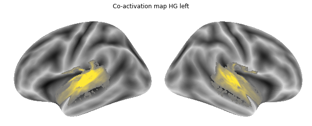
While all of these outputs are very informative and contain important outcomes, we will use only that image most related to our question, i.e. the HG_left_seed_association-test_z_FDR_0.01.nii.gz image. However, you can familiarize yourself with the different outcomes via the Neurosynth FAQ. In order to visualize the co-activation map, we will define a small function relying on nilearn plotting tools:
def plot_meta_analyses_map(meta_analyses_map, roi=None, interactive=False, surface=True, coactivation=True):
fs_average = datasets.fetch_surf_fsaverage('fsaverage')
if coactivation:
title = ' '.join(meta_analyses_map[meta_analyses_map.rfind('/')+1:meta_analyses_map.rfind('_seed')].split('_'))
title = 'Co-activation map %s' %title
else:
title = meta_analyses_map[meta_analyses_map.rfind('p-')+2:meta_analyses_map.rfind('_s')]
title = 'neuroquery meta-analyses map %s' %title
ac_masker = NiftiMasker(mask_img=ac_mask)
meta_analyses_map_ac_data = ac_masker.fit_transform(meta_analyses_map)
meta_analyses_map = ac_masker.inverse_transform(meta_analyses_map_ac_data)
if surface is False and interactive is False:
fig = plot_img(meta_analyses_map, threshold=0.1, bg_img=datasets.load_mni152_template(),
cmap='cividis', draw_cross=False, colorbar=True, title=title)
if roi:
fig.add_contours(roi, levels=[0],
colors='black',
filled=False)
elif surface is True and interactive is False:
hemis= ['left', 'right']
modes = ['lateral']
aspect_ratio=1.4
surf = {
'left': fs_average['infl_left'],
'right': fs_average['infl_right'],
}
texture = {
'left': vol_to_surf(meta_analyses_map, fs_average['pial_left']),
'right': vol_to_surf(meta_analyses_map, fs_average['pial_right'])
}
figsize = plt.figaspect(len(modes) / (aspect_ratio * len(hemis)))
fig, axes = plt.subplots(nrows=len(modes),
ncols=len(hemis),
figsize=figsize,
subplot_kw={'projection': '3d'})
axes = np.atleast_2d(axes)
for index_mode, mode in enumerate(modes):
for index_hemi, hemi in enumerate(hemis):
bg_map = fs_average['sulc_%s' % hemi]
plot_surf_stat_map(surf[hemi], texture[hemi],
view=mode, hemi=hemi,
bg_map=bg_map,
axes=axes[index_mode, index_hemi],
colorbar=False, # Colorbar created externally.
threshold=0.0001,
cmap='cividis')
for ax in axes.flatten():
# We increase this value to better position the camera of the
# 3D projection plot. The default value makes meshes look too small.
ax.dist = 6
fig.subplots_adjust(wspace=-0.02, hspace=0.0)
fig.suptitle(title)
elif surface is False and interactive is True:
fig = view_img(meta_analyses_map, cmap="cividis", threshold=0.0001, black_bg=False, colorbar=True,
draw_cross=False, bg_img=datasets.load_mni152_template(), title=title)
elif surface is True and interactive is True:
fig = view_img_on_surf(meta_analyses_map, cmap="cividis", threshold=0.0001, black_bg=False,
colorbar=False, surf_mesh=fs_average, title=title)
Let’s use it to plot the co-activation map we just computed, namely the one for the left HG:
plot_meta_analyses_map('/data/mvs/derivatives/meta_analyses/results/neurosynth_maps/HG_left_seed_association-test_z_FDR_0.01.nii.gz', HG_left,
interactive=False, surface=True)
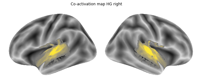
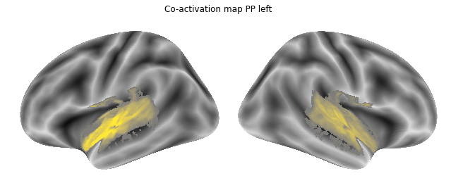
As we have everything we need in place, we can compute the co-activation maps for all ROIs using a small for-loop:
for roi, roi_name in zip(list_rois, list_rois_names):
network.coactivation(neurosynth_dataset, roi, output_dir=opj(results_path, 'neurosynth_maps'), prefix='%s_seed' %roi_name)
Checking our results path, we should now have co-activation maps for each ROI:
coactivation_maps = glob(opj(results_path, 'neurosynth_maps', '*_association-test_z_FDR_0.01.nii.gz'))
coactivation_maps.sort()
coactivation_maps
['/data/mvs/derivatives/meta_analyses/results/neurosynth_maps/HG_left_seed_association-test_z_FDR_0.01.nii.gz',
'/data/mvs/derivatives/meta_analyses/results/neurosynth_maps/HG_right_seed_association-test_z_FDR_0.01.nii.gz',
'/data/mvs/derivatives/meta_analyses/results/neurosynth_maps/PP_left_seed_association-test_z_FDR_0.01.nii.gz',
'/data/mvs/derivatives/meta_analyses/results/neurosynth_maps/PP_right_seed_association-test_z_FDR_0.01.nii.gz',
'/data/mvs/derivatives/meta_analyses/results/neurosynth_maps/PT_left_seed_association-test_z_FDR_0.01.nii.gz',
'/data/mvs/derivatives/meta_analyses/results/neurosynth_maps/PT_right_seed_association-test_z_FDR_0.01.nii.gz',
'/data/mvs/derivatives/meta_analyses/results/neurosynth_maps/aSTG_left_seed_association-test_z_FDR_0.01.nii.gz',
'/data/mvs/derivatives/meta_analyses/results/neurosynth_maps/aSTG_right_seed_association-test_z_FDR_0.01.nii.gz',
'/data/mvs/derivatives/meta_analyses/results/neurosynth_maps/pSTG_left_seed_association-test_z_FDR_0.01.nii.gz',
'/data/mvs/derivatives/meta_analyses/results/neurosynth_maps/pSTG_right_seed_association-test_z_FDR_0.01.nii.gz']
Jop, all there. Let’s plot them:
for roi_map in coactivation_maps:
plot_meta_analyses_map(roi_map, interactive=False, surface=True)

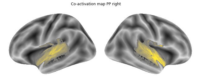

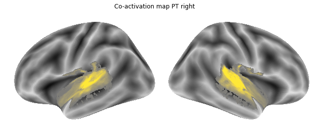
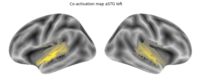
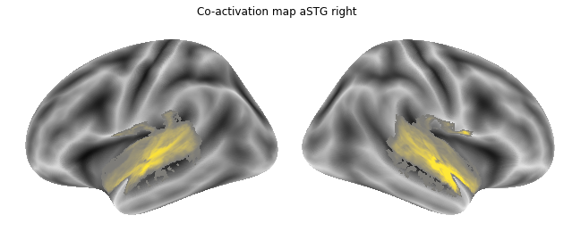
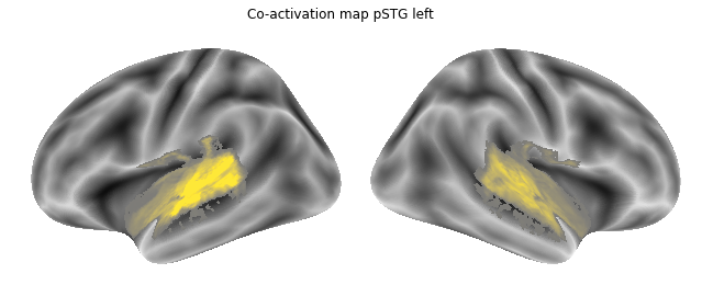
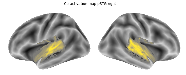
That already concludes the final step of the co-activation analyses, as neurosynth made it super easy and straightforward to compute these maps. Next up, we will use Neuroquery to obtain meta-analytic maps for each of our conditions.
Condition specific meta-analytic maps
While the previous step used meta-analyses to investigate the proposed functional principles by means of ROI co-activation, we can also apply a different meta-analytic approach to do so, which will additionally allow us to relate the outcomes even more directly to our study. This refers to condition specific meta-analytic maps and means that we are going to use meta-analyses to obtain maps for our included conditions voice, singing and music. Given that neurosynth does include a set of pre-computed terms which do not entail singing, we will use Neuroquery to obtain these maps as it allows arbitrary queries that are subsequently mapped to a controlled vocabulary. Overall, it works comparably to neurosynth: at first, we need to initiate a dataset or in this case a model:
encoder = NeuroQueryModel.from_data_dir(fetch_neuroquery_model())
We can now define an arbitrary query in text form, for example: music:
query = """Music"""
and apply the Neuroquery model to it:
nq_music = encoder(query)
The output is a dictionary that contains the meta-analytic map in different form, words that are similar or related to our query and the corresponding studies:
nq_music
{'brain_map': <nibabel.nifti1.Nifti1Image at 0x7fa64d429160>,
'z_map': <nibabel.nifti1.Nifti1Image at 0x7fa64d429160>,
'raw_tfidf': <1x6308 sparse matrix of type '<class 'numpy.float64'>'
with 1 stored elements in Compressed Sparse Row format>,
'smoothed_tfidf': array([1.19950202e-06, 0.00000000e+00, 0.00000000e+00, ...,
4.03333355e-05, 0.00000000e+00, 0.00000000e+00]),
'similar_words': similarity weight_in_brain_map weight_in_query n_documents
music 0.998861 11.399395 1.0 623
auditory 0.001724 1.035886 0.0 4009
temporal 0.000894 0.306217 0.0 11897
auditory cortex 0.000735 0.192881 0.0 846
cerebellum 0.000269 0.160110 0.0 5578
... ... ... ... ...
fluency 0.000003 0.000000 0.0 1098
fluent 0.000007 0.000000 0.0 524
focal 0.000005 0.000000 0.0 1406
focus 0.000004 0.000000 0.0 5586
zone 0.000040 0.000000 0.0 699
[2951 rows x 4 columns],
'similar_documents': pmid title \
0 15784423 Separate cortical networks involved in music p...
1 22110619 Music and Emotions in the Brain: Familiarity M...
2 16516496 It don't mean a thing…
3 22144968 A Functional MRI Study of Happy and Sad Emotio...
4 16023376 The rewards of music listening: Response and p...
.. ... ...
95 16624581 Cognitive priming in sung and instrumental mus...
96 17709121 A Parietal-Temporal Sensory-Motor Integration ...
97 17603027 A network for audio–motor coordination in skil...
98 23051903 Hyperactivation balances sensory processing de...
99 24790186 Connecting to Create: Expertise in Musical Imp...
pubmed_url similarity
0 https://www.ncbi.nlm.nih.gov/pubmed/15784423 0.876373
1 https://www.ncbi.nlm.nih.gov/pubmed/22110619 0.788177
2 https://www.ncbi.nlm.nih.gov/pubmed/16516496 0.776961
3 https://www.ncbi.nlm.nih.gov/pubmed/22144968 0.766900
4 https://www.ncbi.nlm.nih.gov/pubmed/16023376 0.765290
.. ... ...
95 https://www.ncbi.nlm.nih.gov/pubmed/16624581 0.265929
96 https://www.ncbi.nlm.nih.gov/pubmed/17709121 0.257820
97 https://www.ncbi.nlm.nih.gov/pubmed/17603027 0.234380
98 https://www.ncbi.nlm.nih.gov/pubmed/23051903 0.233563
99 https://www.ncbi.nlm.nih.gov/pubmed/24790186 0.231366
[100 rows x 4 columns],
'highlighted_text': '<highlighted_text><extracted_phrase standardized_form="music" in_model="true">Music</extracted_phrase></highlighted_text>'}
As the map is Nifti1Image, we can easily save it in our results path:
nq_music['brain_map'].to_filename(opj(results_path, 'neuroquery_maps/neurquerymap-music_space-MNI152NLin2009cAsym.nii.gz'))
nq_music_map = glob(opj(results_path, 'neuroquery_maps/neurquerymap-music_space-MNI152NLin2009cAsym.nii.gz'))[0]
nq_music_map
'/data/mvs/derivatives/meta_analyses/results/neuroquery_maps/neurquerymap-music_space-MNI152NLin2009cAsym.nii.gz'
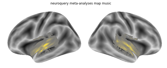
Using our plotting function from before we can check the map:
plot_meta_analyses_map(nq_music_map, interactive=False, surface=True, coactivation=False)
The words that are similar or related to our query are stored in a Dataframe and can thus be checked without problem:
print(nq_music["similar_words"].head(10))
similarity weight_in_brain_map weight_in_query n_documents
music 0.998861 11.399395 1.0 623
auditory 0.001724 1.035886 0.0 4009
temporal 0.000894 0.306217 0.0 11897
auditory cortex 0.000735 0.192881 0.0 846
cerebellum 0.000269 0.160110 0.0 5578
premotor 0.001050 0.130237 0.0 3200
motor 0.000259 0.129558 0.0 7928
sound 0.000679 0.110710 0.0 2261
parahippocampal 0.000360 0.108145 0.0 3512
superior 0.000596 0.087512 0.0 9978
The same holds true for the corresponding studies:
print(nq_music["similar_documents"].head(10))
pmid title \
0 15784423 Separate cortical networks involved in music p...
1 22110619 Music and Emotions in the Brain: Familiarity M...
2 16516496 It don't mean a thing…
3 22144968 A Functional MRI Study of Happy and Sad Emotio...
4 16023376 The rewards of music listening: Response and p...
5 25309407 Moving to Music: Effects of Heard and Imagined...
6 22114191 Long-term music training tunes how the brain t...
7 23274514 Neural correlates of music recognition in Down...
8 27084302 LSD modulates music-induced imagery via change...
9 23107380 Mentalising music in frontotemporal dementia
pubmed_url similarity
0 https://www.ncbi.nlm.nih.gov/pubmed/15784423 0.876373
1 https://www.ncbi.nlm.nih.gov/pubmed/22110619 0.788177
2 https://www.ncbi.nlm.nih.gov/pubmed/16516496 0.776961
3 https://www.ncbi.nlm.nih.gov/pubmed/22144968 0.766900
4 https://www.ncbi.nlm.nih.gov/pubmed/16023376 0.765290
5 https://www.ncbi.nlm.nih.gov/pubmed/25309407 0.762422
6 https://www.ncbi.nlm.nih.gov/pubmed/22114191 0.734953
7 https://www.ncbi.nlm.nih.gov/pubmed/23274514 0.733976
8 https://www.ncbi.nlm.nih.gov/pubmed/27084302 0.728159
9 https://www.ncbi.nlm.nih.gov/pubmed/23107380 0.724319
We can do the same for the other conditions, starting with voice:
query = """Voice"""
nq_voice = encoder(query)
nq_voice['brain_map'].to_filename(opj(results_path, 'neuroquery_maps/neurquerymap-voice_space-MNI152NLin2009cAsym.nii.gz'))
nq_voice_map = glob(opj(results_path, 'neuroquery_maps/neurquerymap-voice_space-MNI152NLin2009cAsym.nii.gz'))[0]
nq_voice_map
'/data/mvs/derivatives/meta_analyses/results/neuroquery_maps/neurquerymap-voice_space-MNI152NLin2009cAsym.nii.gz'
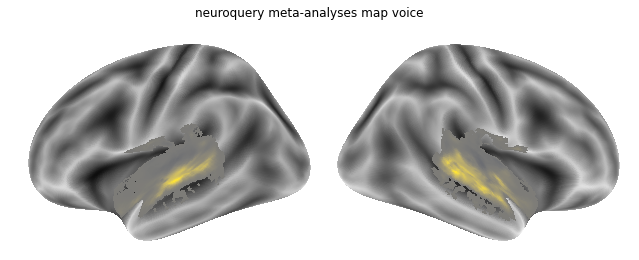
How does the neuroquery meta-analytic map for voice look like?
plot_meta_analyses_map(nq_voice_map, interactive=False, surface=True, coactivation=False)
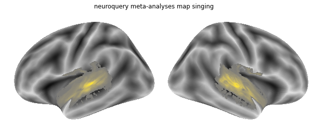
Last but not least: singing.
query = """Singing"""
nq_singing = encoder(query)
nq_singing['brain_map'].to_filename(opj(results_path, 'neuroquery_maps/neurquerymap-singing_space-MNI152NLin2009cAsym.nii.gz'))
nq_singing_map = glob(opj(results_path, 'neuroquery_maps/neurquerymap-singing_space-MNI152NLin2009cAsym.nii.gz'))[0]
nq_singing_map
'/data/mvs/derivatives/meta_analyses/results/neuroquery_maps/neurquerymap-singing_space-MNI152NLin2009cAsym.nii.gz'
And we plot this map as well:
plot_meta_analyses_map(nq_singing_map, interactive=False, surface=True, coactivation=False)
Having obtained a meta-analyses based map for each condition, we can do two things: (1) evaluating if they reflect the proposed functional principles given their assumed spectrotemporal modulations and (2) compare them to the searchlight and gradient maps we computed in the previous steps to check if they carry condition specific information that is generalizable to a certain extent. The latter will be conducted in the next step.
Meta-analytic map - searchlight/gradient comparison
Throughout the last two decades, large scale meta-analyses and datasets it became more and more apparent that the majority of results exhibit a non-existent or heavily restricted generalizability beyond the utilized group of participants and study design/paradigm at hand. Being grounded in a prominent stimulus and task dependency, insights concerning a certain cognitive function or process can vary tremendously across studies and quite often even contradict one another. The processing of auditory information and thus the presumed functional principles of the auditory cortex are no exception to that. While we cannot overcome/address this directly, as we would need to measure a lot of participants with a lot of stimuli and tasks, we can deploy meta-analyses to get a first glimpse. In more detail and applied to our study, we can use the condition specific meta-analyses maps from Neuroquery and compare them to the maps we computed within our dataset, that is searchlight and gradient maps. This should provide us with insights concerning condition specific information that our maps might carry and if they are generalizable to a certain extent (by means of maps computed through large-scale meta-analyses). Prior studies comparing different maps frequently computed the correlation between them. The problem with this approach is that it leads to inflated p-values given the spatial autocorrelation between voxels and thus non-independence in brain maps. To account for this, recent work introduced spatial null models that allow to access the significance of a correlation between two brain maps through permutations. The basic idea or null hypothesis is that if two brain maps are correlated/related in terms of their topography, spatially altering one should result in lower correlation values than in the original one. Via repeating this n times a distribution of correlation values can be obtained to which the original correlation can be compared to. However, there are some caveats with this approach which are grounded in the very idea of it: spatial autocorrelation. When creating spatial null models based on random permutations, the spatial autocorrelation between voxels is destroyed and with it the distinct characteristics of the topography of a map. Thus no claims regarding the comparison of the topography can be made. In order to enable this, spatial null models within which the spatial autocorrelation is preserved during permutations are needed. There are several methods that implement this, for example Spin permutations and Moran Spectral Randomization. Here, we decided to use surrogate maps as introduced in (REF), because they support both volume based and non-whole brain coverage maps. This was crucial as our maps are in volume format and restricted to our auditory cortex mask. Luckily, the BrainSmash toolbox that supports this approach was just introduced. In more detail, we will use it to compare brain maps of interest (our searchlight and gradient maps) to target brain maps (i.e. neuroquery maps). The respective analyses were divided into two steps: creating spatial null models (i.e. surrogate maps of the target brain map) and computing the correlation between maps.
Spatial null models
As mentioned above, we need to create spatial null models, i.e. permuted maps that preserve the spatial autocorrelation of the original map (target brain map). In oder to incorporate the spatial autocorrelation into the permutation, we need respective spatial information, more precisely the distance between voxels that are part of our maps. Here this refers to the distance between voxels within our auditory cortex mask. So far, we used this mask in a bilateral manner, meaning we have both hemispheres in one mask:
sns.set_style('white')
plt.rcParams["font.family"] = "Arial"
fig=plt.figure(num=None, figsize=(12, 6))
ac_mask_both = plot_anat(cut_coords=[-55, -34, 7], figure=fig, draw_cross=False)
ac_mask_both.add_contours(ac_mask,
levels=[0], colors='black')
plt.text(-255, 90, 'Auditory cortex mask both hemispheres',
fontsize=20)
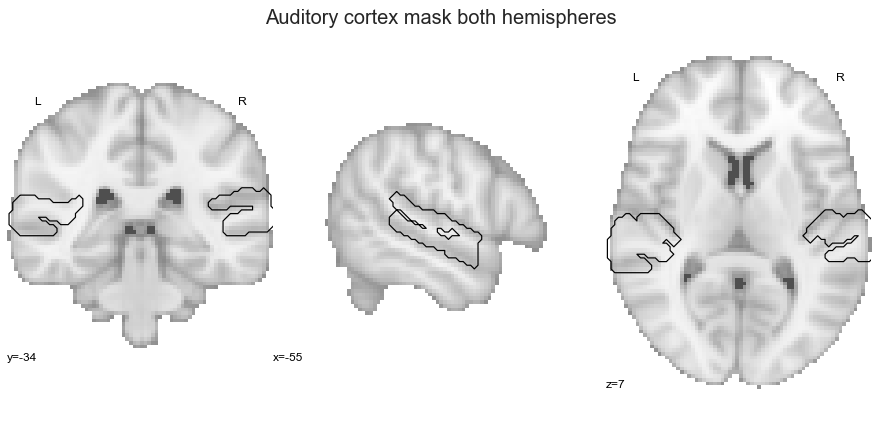
Given that we are talking about spatial autocorrelation and distance between voxels, we should however compute this for each hemisphere separately. Thus, we need to gather the hemisphere specific auditory cortex masks we created in the Auditory Cortex working model section:
ac_mask_left = opj(roi_mask_path, 'tpl-MNI152NLin6Sym_res_02_desc-ACleft_mask.nii.gz')
ac_mask_right = opj(roi_mask_path, 'tpl-MNI152NLin6Sym_res_02_desc-ACright_mask.nii.gz')
We are going to ensure that we cover the area as we did with our bilateral mask:
sns.set_style('white')
plt.rcParams["font.family"] = "Arial"
fig=plt.figure(num=None, figsize=(12, 6))
ac_mask_both = plot_anat(cut_coords=[-55, -34, 7], figure=fig, draw_cross=False)
ac_mask_both.add_contours(ac_mask_left, linewidths=2,
levels=[0], colors=sns.color_palette('cividis', 5).as_hex()[0])
ac_mask_both.add_contours(ac_mask_right, linewidths=2,
levels=[0], colors=sns.color_palette('cividis', 5).as_hex()[4])
roi_legend = [Line2D([0], [0], color=sns.color_palette('cividis', 5)[0], lw=9, label='AC mask left'),
Line2D([0], [0], color=sns.color_palette('cividis', 5)[4], lw=9, label='AC mask right')]
plt.legend(handles=roi_legend, bbox_to_anchor=(-0.07,-0.1), loc="right", ncol=2, prop={'size': 14}, frameon=False)
plt.text(-250, 90, 'Auditory cortex mask per hemisphere',
fontsize=20)
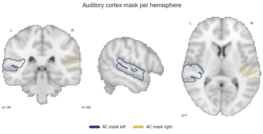
Looks good, so let’s start with the voxel distance computation for the left hemisphere. At first, we need to load the mask and check the shape, as well as unique values of the data:
ac_mask_left_values = load_img(ac_mask_left)
print('The shape of the data is ', ac_mask_left_values.shape)
print('It has the following unique value: ', np.unique(ac_mask_left_values.get_fdata()))
The shape of the data is (91, 109, 91)
It has the following unique value: [0. 1.00000006]
As with most other binary masks, we have 0 and 1 indicating voxels that are not included and those that are. We need to get the coordinates of the latter voxels and can do that via numpy. Please note, we are operating on a 3D image and thus need the respective coordinates in x, y and z:
coord_x_left, coord_y_left, coord_z_left = np.where(ac_mask_left_values.get_fdata() == np.unique(ac_mask_left_values.get_fdata())[1])
print('Number of x coordinates: ', coord_x_left.shape)
print('Number of y coordinates: ', coord_y_left.shape)
print('Number of z coordinates: ', coord_z_left.shape)
Number of x coordinates: (2343,)
Number of y coordinates: (2343,)
Number of z coordinates: (2343,)
Next, we are going to bring them back together, stacking them across x, y and z:
voxel_coords_left = np.vstack([coord_x_left, coord_y_left, coord_z_left]).T
voxel_coords_left.shape
(2343, 3)
Given that the coordinates so far in voxel space, but we need them in reference space, a transformation is required. To do this end, we will apply the affine of the auditory cortex mask to our coordinates using nibabel:
voxel_coords_left = nb.affines.apply_affine(ac_mask_left_values.affine, voxel_coords_left)
voxel_coords_left.shape
(2343, 3)
With that we are ready to compute the distance between voxels, which we can do via scipy’s spatial.distance module, more precisely pdist, using euclidean as the metric:
ac_dist_left= pdist(voxel_coords_left, metric='euclidean')
ac_dist_left.shape
(2743653,)
As a result, we get the distance between all voxels in the left auditory cortex mask, that is the distance between a given voxel and all other voxels. To bring it a more comprehensible form and also the one we will need later on, we will convert this 1D array into a square matrix or voxel by voxel distance matrix using scipy's squareform:
ac_dist_left = squareform(ac_dist_left)
ac_dist_left.shape
(2343, 2343)
Checks out, nice. Before we plot this voxel by voxel distance matrix, let’s do the same for the right hemisphere so that we can plot both side by side:
ac_mask_right_values = load_img(ac_mask_right)
coord_x_right, coord_y_right, coord_z_right = np.where(ac_mask_right_values.get_fdata() == np.unique(ac_mask_right_values.get_fdata())[1])
voxel_coords_right = np.vstack([coord_x_right, coord_y_right, coord_z_right]).T
voxel_coords_right = nb.affines.apply_affine(ac_mask_right_values.affine, voxel_coords_right)
ac_dist_right= squareform(pdist(voxel_coords_right, metric='euclidean'))
ac_dist_right.shape
(2313, 2313)
Coolio, now to the plot. As done throughout all sections we will define a small function that supports both non-interactive and interactive graphics:
def plot_voxel_distance_matrix(dist_mat_left, dist_mat_right, interactive=False):
if interactive is False:
sns.set_style('white')
plt.rcParams["font.family"] = "Arial"
fig, axes = plt.subplots(1,2, figsize = (22, 10))
plot_matrix(dist_mat_left, cmap='cividis', axes=axes[0])
axes[0].set_xlabel('<-- Auditory cortex voxels -->', fontsize=20)
axes[0].set_xticklabels([''])
axes[0].set_ylabel('<-- Auditory cortex voxels -->', fontsize=20)
axes[0].set_yticklabels([''])
axes[0].set_title('left hemisphere', fontsize=20)
plt.subplots_adjust(wspace=0.4)
plot_matrix(dist_mat_right, cmap='cividis', axes=axes[1], colorbar=False)
axes[1].set_xlabel('<-- Auditory cortex voxels -->', fontsize=20)
axes[1].set_xticklabels([''])
axes[1].yaxis.set_label_position("right")
axes[1].set_ylabel('<-- Auditory cortex voxels -->', fontsize=20)
axes[1].set_yticklabels([''])
axes[1].set_title('right hemisphere', fontsize=20)
fig.suptitle('Voxel by voxel euclidean distance within the auditory cortex mask', size=25)
plt.show()
else:
from plotly.subplots import make_subplots
fig = make_subplots(rows=1, cols=2,
subplot_titles=('left hemisphere', 'right hemisphere'),
horizontal_spacing=0.18)
fig.add_trace(go.Heatmap(z=dist_mat_left[:630,:630],
colorscale='cividis',colorbar_x=0.46, transpose=True), row=1, col=1)
fig.add_trace(go.Heatmap(z=dist_mat_right[:630,:630],
colorscale='cividis', showscale = False, transpose=True), row=1, col=2)
fig.update_layout(
autosize=False,
width=900,
height=600,)
fig['layout'].update(template='simple_white')
fig.update_layout(
title={
'text': "Voxel by voxel euclidean distance within the auditory cortex mask",
'y':0.93,
'x':0.5,
'xanchor': 'center',
'yanchor': 'top'})
fig['layout']['xaxis']['title']='<-- Auditory cortex voxels -->'
fig['layout']['xaxis2']['title']='<-- Auditory cortex voxels -->'
fig['layout']['yaxis']['title']='<-- Auditory cortex voxels -->'
fig['layout']['yaxis2']['title']='<-- Auditory cortex voxels -->'
fig['layout']['yaxis']['autorange'] = "reversed"
fig['layout']['yaxis2']['autorange'] = "reversed"
fig['layout']['yaxis2']['side'] = "right"
init_notebook_mode(connected=True)
plot(fig, filename = 'voxel2voxel_dist.html')
display(HTML('voxel2voxel_dist.html'))
Applied to our computed voxel by voxel distance matrices, this is how things look like:
plot_voxel_distance_matrix(ac_dist_left, ac_dist_right, interactive=True)