Preprocessing & individual level statistics
Hereinafter, we will provide the code and steps conducted during the preprocessing and individual level statistical analyses”. Please note, that due to an absent consent of the participants, this page provides the code but you can’t rerun the analyses on the raw data (as mentioned here).
The following steps were run:
structural preprocessing
functional preprocessing
individual level statistics
native space - template space coregistration
native to template space transformation
The respective sections contain further information regarding the specifics and implementation. Let’s start the adventure with structural preprocessing.
Structural preprocessing
The first step of our preprocessing consisted of a comprehensive structural processing pipeline called Mindboggle. It’s aim is to extract a multitude of so called shape features that describe cortical gray matter parts of the brain through volume and surface based characteristics. This entails: volume, thickness, curvature, travel depth, etc. and is obtained for each ROI in the Mindboggle DKT atlas. To this end, mindboggle combines FreeSurfer’s recon-all, ANTs antsCorticalThickness and mindboggle itself via nipype. For this project we utilized exclusively the FreeSurfer output, while the other outputs will be used in subsequent studies. Thus, we don’t go into further details here, but point interested readers to the original mindboggle publication and the mindboggle website. As mindboggle is intended to run as a BIDS app and because it’s a great idea in general, we used the mindboggle docker image to process the structural images. As you can see below, we simply defined the required directories on our host machine and within the docker image, as well as a list of participants to process. Then, we set up a small for loop that applies the mindboggle123 pipeline for a given participant. Please note, that this part is run within the bash shell and not python as we need to run docker.
%%bash

HOST=/data/mvs/
DOCK=/home/jovyan/work

declare -a participants=("sub-01" "sub-02" "sub-03" "sub-04" "sub-05" "sub-06" "sub-07" "sub-08" "sub-09" "sub-10" "sub-11" "sub-12" "sub-13" "sub-14" "sub-15" "sub-16" "sub-17" "sub-18" "sub-19" "sub-20" "sub-21" "sub-22" "sub-23" "sub-24")

for part in "${participants[@]}"
do

    IMAGE=/home/jovyan/work/$part/anat/$part"_T1w.nii.gz"
    ID=$part

    docker run --rm -ti -v $HOST:$DOCK nipy/mindboggle mindboggle123 $IMAGE --id $ID

done
After a good while (geez, a gooooood while), we’ll have our outputs under /data/mvs/derivatives/mindboggle. Within this folder, three subdirectories can be found, corresponding to the included pipelines mindboggle combines: FreeSurfer, ANTs and mindboggle. As said before, we will only use FreeSurfer output hereinafter. Thanks to BIDS and the great community behind it, this first part of the preprocessing was a no-brainer and super straightforward. The subsequent coregistration of the anatomical images and template image was a bit more work, but still feasible given nipype. We will check that next.
Functional preprocessing
The preprocessing of the functional images was roughly divided into two sections: classic preprocessing steps and mask generation. The corresponding steps and functions were conducted in various software packages, including SPM, FSL and FreeSurfer and implemented, connected and run via nipype. The “classic” preprocessing entailed realignment (through SPM’s Realign), coregistration (through FreeSurfer’s BBRegister) and spatial smoothing (through SPM’s Smooth). The mask creation part contained the creation of participant specific masks aimed to restrict the subsequent statistical analyses to cortical gray matter voxels. First, we used FreeSurfer’s Binarize to extract and combine cortical gray matter voxels belonging to either the left or right hemisphere from FreeSurfer’s aparc+aseg volume (which we obtained within the structural processing) and binarized the resulting image. Next, we transformed this image to a given participant’s functional space by using the computed coregistration matrix within FreeSurfer’s ApplyVolTransform. Subquently, we used FSL’s ImageMaths to substract the transformed cortical gray matter mask from the mean functional image (obtained through the realign step) which yielded a mask in a given participant’s functional space that was covered by the data acquisition protocols FoV and restricted to gray matter. In the last step, the resulting mask was dilated by one voxel and binarized (both via FreeSurfer’s Binarize). Hereinafter we show how this was set up, including important paths and variables, necessary nodes and workflow definition. However, as usual we start with the important of the recquired modules and functions.
Import modules
As mentioned before, we’ll use the nipype implementation of the respective functions to allow for easy and reproducible execution.
from os.path import join as opj
from nipype.interfaces.freesurfer import (BBRegister, ApplyVolTransform,
                                          Binarize, MRIConvert, FSCommand)
from nipype.interfaces.fsl import BET, BinaryMaths, ImageMaths
from nipype.interfaces.spm import (Realign, Smooth, SPMCommand)
from nipype.interfaces.utility import Function, IdentityInterface
from nipype.interfaces.io import FreeSurferSource, SelectFiles, DataSink
from nipype.algorithms.rapidart import ArtifactDetect
from nipype.algorithms.misc import Gunzip
from nipype.pipeline import Node, MapNode, Workflow
Define and set important paths and variables
At first, we need to define a few important paths and variables that are needed for various aspects of the workflow. For example, we need to tell nipype where our SPM installation is. Notably, we set up the standalone version which doesn’t require MATLAB as it can run via its compiler runtime.
matlab_cmd = '/usr/local/spm12/run_spm12.sh /usr/local/MATLAB/MATLAB_Compiler_Runtime/v713/'
SPMCommand.set_mlab_paths(matlab_cmd=matlab_cmd, use_mcr=True)
We also need to set the data directory and list of participants to process:
experiment_dir = '/data/mvs/'
data_dir= experiment_dir

participant_list = []

for i in range(1,24):
    if i < 10:
        participant_list.append('sub-0%s' %i)
    else:
        participant_list.append('sub-%s' %i)
We’re only missing the output and working directory of the workflow:
output_dir = '/data/mvs/derivatives/preprocessing'
working_dir = '/data/mvs/derivatives/preprocessing/workingdir_preprocessing'
Now that we have that, we can define our workflow nodes:
Define and set processing nodes
We need to set up one node for each of the above mentioned functions. Within that, we can additionally specify certain aspects of how the respective functions should run. Initially, we actually need a utility function to unzip our functional images as SPM can’t read zipped files. The Gunzip function allows us to do that:
gunzip = MapNode(Gunzip(), name="gunzip", iterfield=['in_file'])
Next, the unzipped files should be realigned through SPM’s Realign. Here, we set the parameter register_to_mean to True as we want to apply a two-step realignment procedure. This means that the first image of the second run was realigned to the first image of the first run and subsequently all images of a given run were realigned to the first image of their respective run.
realign = Node(Realign(register_to_mean=True),
               name="realign")
The coregistration of a participant’s functional and structural space was computed via FreeSurfer’s BBRegister and set up to use an SPM affine initiation and an optimization for T2w images.
bbregister = Node(BBRegister(init='spm',
                             contrast_type='t2',
                             out_fsl_file=True),
                  name='bbregister')
Functional images were spatially smoothed with a 6mm FHWM Gaussian Kernel using SPM’s Smooth.
smooth = Node(Smooth(fwhm=6),
              name="smooth")
Through FreeSurfer’s Binarize function labels corresponding cortical gray matter in the left and right hemisphere were extracted from each participant’s aparc+aseg volume obtained through recon-all running as part of mindboggle. As you can see, this refers to label 3 and 42.
binarizeCortical = Node(Binarize(out_type='nii.gz',
                                    match = [3,42],
                                    binary_file='binarized_cortical_gm.nii.gz'),
                        name='binarizeCortical')
The resulting binary mask needs to be transformed into a given participant’s native space. We can do that with FreeSurfer’s ApplyVolTransform, setting the interpolation method to nearest.
applyVolTrans_cortical_mask = Node(ApplyVolTransform(
                                  interp='nearest'),
                name='applyVolTrans_cortical_mask')
Now that the structural cortical gray matter mask is in functional space, we need to create a binary mask from the functional images to build their intersection. As we will get the mean functional image through the realign step, we can use FSL’s BET to compute a binary mask from it while restricting our image to cortical voxels only. Thus, we specify mask=True within the function definition and additionally set robust to true in order to run multiple iterations of the mask extraction, enhancing the fit of our results. Regarding fit we also set the frac parameter, here to a value of 0.55, which defines the strictness of the extraction.
meanfuncmask = Node(interface=BET(mask=True,
                                  no_output=False,
                                  frac=0.55,
                                  robust=True,
                                  output_type='NIFTI',
                                  out_file='meanfunc'),
                       name='meanfuncmask')
With that we have both, a structural cortical gray matter mask and a functional cortical mask, in the same space and can subtract them from one another to build their intersection. The result will be a mask in a given participant’s functional space that was covered by the data acquisition protocols FoV and restricted to gray matter. We can achieve this via FSL’s ImageMaths defining the operation (op_string) as -mas. Note that we set it up as a MapNode and defining the in_file as the iterfield, thus enabling multiple input files.
subtract_cortical_gm_func = MapNode(interface=ImageMaths(op_string='-mas',
                                                    output_type='NIFTI',
                                                    out_file='cortical_gm_func_mask.nii'),
                                    iterfield=['in_file'],
                                    name='subtract_cortical_gm_func')
As there’s always some uncertainty when it comes to segmentation, extraction and transformation, we’re going to dilate the resulting mask by one voxel and binarize it again. Here, FreeSurfer’s Binarize comes in handy again.
dilate_binarize_mask = Node(Binarize(dilate=1,
                          min=0.5),
              name='dilate_binarize_mask')
That’s it, all necessary processing nodes are set and defined. Now we need to create a workflow and connect them.
Create the workflow and connect nodes
In order to connect our processing nodes and run them as a workflow, we need to create the basis via defining an empty workflow and setting the base directory within which the processing will occur. In our case the workflow is called preproc_mvs and the directory will be the working_dir within our experiment_dir we defined in the beginning.
preproc_mvs = Workflow(name='preproc_mvs')
preproc_mvs.base_dir = opj(experiment_dir, working_dir)
Within this empty workflow we can now connect our processing nodes in the desired order, defining inputs and outputs as necessary. To enable a better understanding, we added some inline comments.
preproc_mvs.connect([(gunzip, realign, [('out_file', 'in_files')]), # send unzipped files to realignment node
                     (realign, meanfuncmask, [('mean_image', 'in_file')]), # create a skull stripped binarized mask image from the mean functional image
                     (realign, bbregister, [('mean_image', 'source_file')]), # coregister mean functional image and anatomical image
                     (realign, smooth, [('realigned_files', 'in_files')]), # send realigned files to smooth node
                     (binarizeCortical, applyVolTrans_cortical_mask, [('binary_file', 'source_file')]), # transform cortical gray matter mask to functional space, antomical space is source
                     (realign, applyVolTrans_cortical_mask, [('mean_image', 'target_file')]), # transform cortical gray matter mask to functional space, functional space is target
                     (bbregister, applyVolTrans_cortical_mask,[('out_reg_file','reg_file')]), # transform cortical gray matter mask to functional space, use computed coregistration
                     (meanfuncmask, subtract_cortical_gm_func, [('mask_file', 'in_file')]), # create a combined mask from the anatomical cortical gray matter and functional mask
                     (applyVolTrans_cortical_mask, subtract_cortical_gm_func, [('transformed_file', 'in_file2')]), # create a combined mask from the anatomical cortical gray matter and functional mask
                     (subtract_cortical_gm_func, dilate_binarize_mask, [('out_file', 'in_file')]), # create a combined mask from the anatomical cortical gray matter and functional mask
                    ])
The workflow in itself is now set up. However, we also need to define input and output streams of the workflow, that is how data enters and leaves. The first part can be done via two parts, the IdentityInterface function and the SelectFiles function. Within the first we set the list participant_list as input to iterate over:
infosource = Node(IdentityInterface(fields=['participant_id']),
                  name="infosource")
infosource.iterables = [('participant_id', participant_list)]
Within the second, we define template paths to the we want to include and operate on. More precisely, this includes the functional images and the aparc_aseg volume:
templates = {'func': '{participant_id}/func/*.nii.gz',
             'aparc_aseg': '/derivatives/mindboggle/freesurfer/{participant_id}/mri/aparc+aseg.mgz'}
selectfiles = Node(SelectFiles(templates,
                               base_directory=experiment_dir),
                   name="selectfiles")
The output stream can be set via the DataSink function, defining the base and output directory respectively.
datasink = Node(DataSink(base_directory=experiment_dir,
                         container=output_dir),
                name="datasink")
As some functions will add some additional identifiers to our filenames, we will in turn add some substitutions to our DataSink function:
substitutions = [('_subject_id_', ''),
                 ('_warped', '')]
datasink.inputs.substitutions = substitutions
So far so good, let’s connect the input and output streams to our workflow.
preproc_mvs.connect([(infosource, selectfiles, [('participant_id', 'participant_id')]), # select files from participants
                     (infosource, bbregister, [('participant_id', 'subject_id')]), # send participant id to bbregister
                     (selectfiles, gunzip, [('func', 'in_file')]), # send functional files to unzip node
                     (selectfiles, binarizeCortical, [('aparc_aseg', 'in_file')]), # extract and binarize cortical gray matter voxels
                     (realign, datasink, [('mean_image', 'realign.@mean'), # send mean image from realignment to datasink
                                          ('realignment_parameters', 'realign.@parameters')]), # send realignment parameters to datasink
                     (binarizeCortical, datasink, [('binary_file', 'masks.@binarized_cortical_gm_mask')]), # send cortical gray matter mask to datasink
                     (meanfuncmask, datasink, [('mask_file', 'masks.@mean_functional_mask')]), # send mean functional mask to datasink
                     (bbregister, datasink, [('out_reg_file', 'bbregister.@out_reg_file'), # send registration file to datasink
                                             ('out_fsl_file', 'bbregister.@out_fsl_file'), # send fsl file to datasink
                                             ('registered_file', 'bbregister.@registered_file')]), # send registered file to datasink
                     (subtract_cortical_gm_func, datasink, [('out_file', 'masks.@cortical_gm_func_mask')]), # send cortical gray matter mask in functional space to datasink
                     (smooth, datasink, [('smoothed_files', 'smooth.@smoothed_files')]), # send smoothed files to datasink
                    ])
Evaluate the workflow
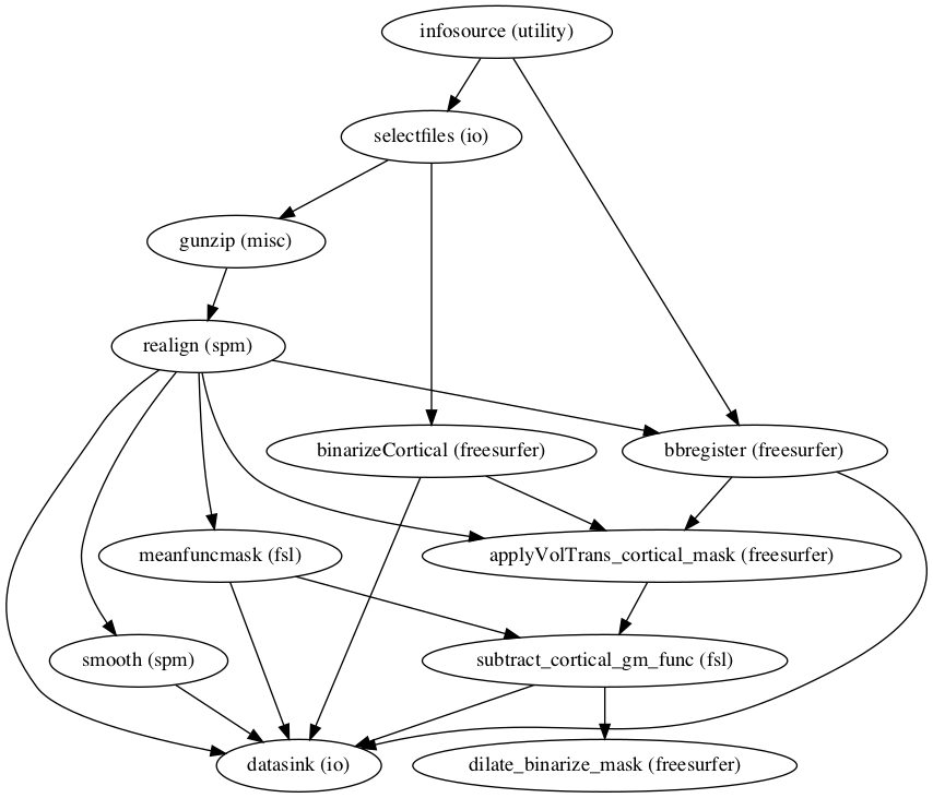
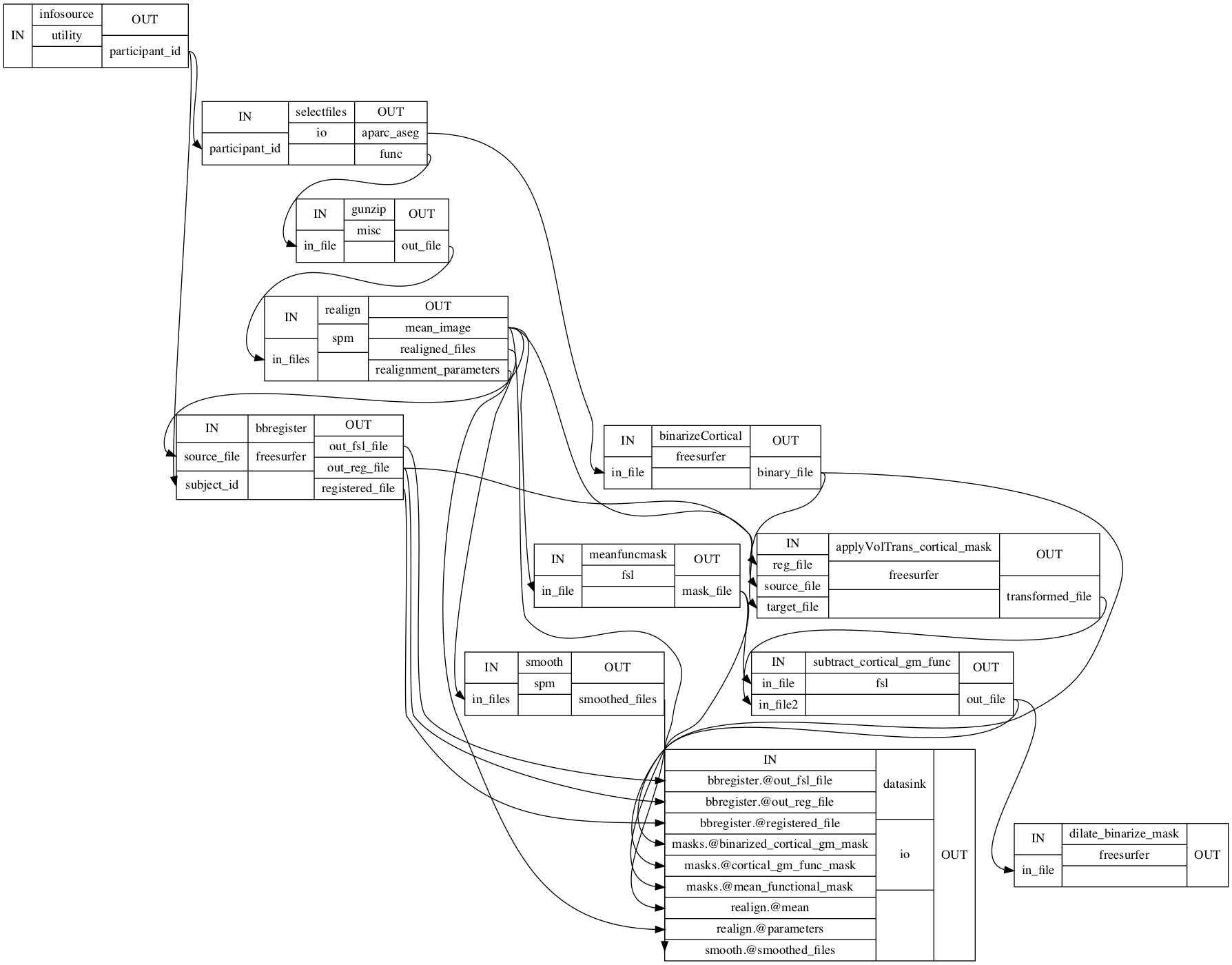
That was a lot of connections, thus we should make sure that everything fits. Luckily, nipype has some inbuilt functionality to visualize workflows. We can even generate two different graphs: one with less detail and one with more detail:
preproc_mvs.write_graph(graph2use='colored', format='png', simple_form=True);

preproc_mvs.write_graph(graph2use='flat', format='png', simple_form=True)
'/data/mvs/derivatives/preprocessing/workingdir_preprocessing/preproc_mvs/graph.png'
The graphs are written to a .png file, but we can use IPython’s Image function to visualize them here:
from IPython.display import Image
Image(filename="/data/mvs/derivatives/preprocessing/workingdir_preprocessing/preproc_mvs/graph.png")
Image(filename="/data/mvs/derivatives/preprocessing/workingdir_preprocessing/preproc_mvs/graph_detailed.png")
Statistical analyses - individual level
Before we start, let’s important the modules and functions we need.
Import Modules
import pandas as pd
from nipype.algorithms.modelgen import SpecifySPMModel
from nipype.interfaces.spm import Level1Design, EstimateModel, EstimateContrast
from nipype.interfaces.freesurfer import MRIConvert
We also need to define new output and working directories as we’re in the next processing stage.
Define and set important paths
output_dir_ind_level = 'individual_statistics'
working_dir_ind_level = 'workingdir_individual_statistics'
experiment_dir = '/data/mvs'
Define and set processing nodes
With our data preprocessed, we can continue to the individual level statistics. In other words, we want to the model the cortical responses to the included stimuli. Please note, that we, in contrast to most pipelines, will run the statistical analyses on the individual level in a given participant’s native functional space instead of a template space. However, we will transform the resulting contrast images to a template space later on. We choose the rather “classic” approach of a mass-univariate analysis in form of a voxel-wise General Linear Model (GLM). We’ll use SPM functionality for that as it includes an option for nicely modelling the autocorrelation in datasets with comparably fast data acquisition protocols. As the TR in our case was 0.529 seconds, this appears appropriate. This part of the analyses contained three steps: defining a model, estimating the model and computing contrasts. As in the preprocessing, we will start with defining the necessary nodes and subsequently connect them within a workflow. We’re going to start with the basic model definition through nipype’s SpecifySPMModel. Given that we don’t want to concatenate runs, we set the concatenate_runs parameter to False. Both input and output units of our model will be in seconds (secs). The TR of our paradigm was 0.529 seconds and we choose a high pass filter cutoff of 128 Hz.
modelspec = Node(SpecifySPMModel(concatenate_runs=False,
                                 input_units='secs',
                                 output_units='secs',
                                 time_repetition=0.529,
                                 high_pass_filter_cutoff=128),
                 name="modelspec")
The next step consists of setting up basics of the design matrix we want to estimate later on. We use SPM’s Level1Design function using the canonical hemodynamic response function and no derivatives. As before our timing units are seconds and our TR was 0.529 seconds. We set the model_serial_correlation parameter to FAST in order to address our comparably fast TR.
level1design = Node(Level1Design(bases={'hrf': {'derivs': [0, 0]}},
                                 timing_units='secs',
                                 interscan_interval=0.529,
                                 model_serial_correlations='FAST'),
                    name="level1design")
Setting up a model is only have of the deal, we also need to actually estimate it. Here, we did that using SPM’s EstimateModel function, choosing the classical estimation method.
level1estimate = Node(EstimateModel(estimation_method={'Classical': 1}),
                      name="level1estimate")
From our estimated model we can compute contrasts, that is comparing the estimated responses to our stimuli against other modeled or unmodeled aspects of our paradigm. SPM’s EstimateContrast comes in handy for that.
conestimate = Node(EstimateContrast(), name="conestimate")
During the preprocessing we needed to unzip our functional files as SPM can’t read zipped files. However, we want to continue with zipped files and thus use FreeSurfer’s MRIConvert as a MapNode to zip the computed contrast images.
mriconvert = MapNode(MRIConvert(out_type='niigz'),
                     name='mriconvert',
                     iterfield=['in_file'])
Nice, the basics are done. Let’s create a workflow and connect the nodes
Create the workflow and connect nodes
As done for the preprocessing, we have to create an empty workflow and connect our processing nodes accordingly. The basics steps are always identical, we just have to adapt the workflow name and experiment as well as working directory.
ind_level = Workflow(name='ind_level')
ind_level.base_dir = opj(experiment_dir, working_dir_ind_level)
Let’s connect our processing nodes:
ind_level.connect([(modelspec, level1design, [('session_info', 'session_info')]), # send model specifiction to individual level model
                   (level1design, level1estimate, [('spm_mat_file', 'spm_mat_file')]), # estimate individual level model
                   (level1estimate, conestimate, [('spm_mat_file', 'spm_mat_file'), # send spm.mat file to contrast estimation
                                                  ('beta_images', 'beta_images'), # send beta images to contrast estimation
                                                  ('residual_image', 'residual_image')]), # send residual image to contrast estimation
                   (conestimate, mriconvert, [('con_images', 'in_file')]) # zip contrast images
                  ])
So far, we’re missing one of the most crucial parts. We’re interested in the responses evoked through our stimuli, however, but we didn’t specify what stimuli where presented where for how long. This information can be found in the events files that describe a given experimental run per participant. Based on our paradigm, each participant has two event files as two runs were presented. Within each we have the trial type, onset and duration for every presented stimulus. Here’s an example of how they look like (note how easy and comprehensive this through BIDS and pandas:
event_file_example = pd.read_table('static/sub-01_task-mvs_run-01_events.tsv')
event_file_example
| trial_type | onset | duration | correct | |
|---|---|---|---|---|
| 0 | Music | 4.710 | 1.87 | Y |
| 1 | Music | 8.726 | 1.76 | Y |
| 2 | Music | 20.776 | 1.68 | Y |
| 3 | Music | 24.792 | 1.76 | Y |
| 4 | Music | 28.809 | 1.57 | Y |
| ... | ... | ... | ... | ... |
| 85 | Voice | 337.496 | 1.39 | Y |
| 86 | Voice | 341.513 | 1.97 | Y |
| 87 | Voice | 353.546 | 1.71 | Y |
| 88 | Voice | 357.562 | 1.43 | Y |
| 89 | Voice | 361.562 | 1.86 | Y |
90 rows × 4 columns
Let’s check each condition separately.
for condition in event_file_example.groupby('trial_type'):
    print(condition)
('Music',    trial_type    onset  duration correct
0       Music    4.710      1.87       Y
1       Music    8.726      1.76       Y
2       Music   20.776      1.68       Y
3       Music   24.792      1.76       Y
4       Music   28.809      1.57       Y
5       Music   52.874      1.45       Y
6       Music   56.874      1.76       Y
7       Music   72.923      2.00       Y
8       Music   84.940      1.85       Y
9       Music   88.939      1.76       Y
10      Music   96.956      1.80       Y
11      Music  100.956      1.65       Y
12      Music  116.972      1.70       Y
13      Music  120.972      1.83       Y
14      Music  129.005      1.67       Y
15      Music  153.087      1.65       Y
16      Music  169.103      1.88       Y
17      Music  181.136      1.72       Y
18      Music  193.185      1.52       Y
19      Music  221.268      1.69       Y
20      Music  233.300      1.60       Y
21      Music  237.300      1.90       Y
22      Music  253.333      1.71       Y
23      Music  285.415      1.48       Y
24      Music  289.415      1.48       Y
25      Music  301.431      1.73       Y
26      Music  317.464      1.73       Y
27      Music  329.480      1.74       Y
28      Music  333.496      1.52       Y
29      Music  349.529      1.76       Y)
('Singing',    trial_type    onset  duration correct
30    Singing   16.759      1.74       Y
31    Singing   32.825      1.50       Y
32    Singing   36.825      1.91       Y
33    Singing   44.858      1.65       Y
34    Singing   48.858      1.14       Y
35    Singing   64.907      1.54       Y
36    Singing   68.924      1.55       Y
37    Singing   76.923      1.92       Y
38    Singing  104.955      2.00       Y
39    Singing  124.988      1.99       Y
40    Singing  137.038      1.50       Y
41    Singing  145.054      1.99       Y
42    Singing  149.070      1.76       Y
43    Singing  161.103      2.15       Y
44    Singing  173.103      1.76       Y
45    Singing  177.119      1.74       Y
46    Singing  185.152      1.31       Y
47    Singing  189.169      1.32       Y
48    Singing  209.235      1.53       Y
49    Singing  213.235      1.74       Y
50    Singing  225.284      1.45       Y
51    Singing  229.284      1.71       Y
52    Singing  241.300      1.31       Y
53    Singing  261.349      1.64       Y
54    Singing  269.366      1.75       Y
55    Singing  273.365      1.51       Y
56    Singing  293.415      1.80       Y
57    Singing  297.414      2.14       Y
58    Singing  305.431      1.72       Y
59    Singing  345.529      1.48       Y)
('Voice',    trial_type    onset  duration correct
60      Voice   12.743      1.51       Y
61      Voice   40.841      1.81       Y
62      Voice   60.891      1.66       Y
63      Voice   80.923      1.79       Y
64      Voice   92.956      1.97       Y
65      Voice  108.955      1.61       Y
66      Voice  112.972      1.88       Y
67      Voice  133.021      1.56       Y
68      Voice  141.037      1.79       Y
69      Voice  157.087      1.67       Y
70      Voice  165.103      1.87       Y
71      Voice  197.185      1.54       Y
72      Voice  201.202      2.13       Y
73      Voice  205.218      1.61       Y
74      Voice  217.251      1.89       Y
75      Voice  245.317      1.72       Y
76      Voice  249.333      1.87       Y
77      Voice  257.349      1.97       Y
78      Voice  265.366      1.58       Y
79      Voice  277.382      1.56       Y
80      Voice  281.398      1.96       Y
81      Voice  309.447      1.66       Y
82      Voice  313.464      1.63       Y
83      Voice  321.464      1.60       Y
84      Voice  325.463      1.39       Y
85      Voice  337.496      1.39       Y
86      Voice  341.513      1.97       Y
87      Voice  353.546      1.71       Y
88      Voice  357.562      1.43       Y
89      Voice  361.562      1.86       Y)
We still need to extract and provide this information within our model. Luckily, fmriflows has a great function we can borrow and adapt to do so. The basic idea is that we provide event files and condition names as input and get the needed information in a so called Bunch.
def collect_model_info(event_files, condition_names):

    import numpy as np
    import pandas as pd
    from nipype.interfaces.base import Bunch

    model_info = []

    for i, f in enumerate(event_files):

        trialinfo = pd.read_csv(f, sep='	')
        stimuli_list = [t for t in trialinfo.trial_type if str(t) in condition_names]
        conditions = []
        onsets = []
        durations = []

        for group in trialinfo.groupby('trial_type'):
            if str(group[0]) in condition_names:
                conditions.append(str(group[0])+'_run-0%s'%str(i+1))
                onsets.append(list(group[1].onset))
                durations.append(group[1].duration.tolist())

        model_info.append(Bunch(conditions=conditions,
                                onsets=onsets,
                                durations=durations))

    return model_info
In order to include this function in our workflow, we need to set up a Function Node that runs our above created function.
get_model_info = Node(Function(input_names=['event_files', 'condition_names'],
                               output_names=['model_info'],
                               function=collect_model_info),
                      name='get_model_info')
get_model_info.inputs.condition_names = ['Music', 'Singing', 'Voice']
Another thing we need to do is defining the contrasts that should be computed after the model was estimated. To this end, we create a list of condition names based on our paradigm, that is music, singing and voice for each of two runs:
condition_names = ['Music_run-01','Singing_run-01','Voice_run-01','Music_run-02','Singing_run-02', 'Voice_run-02']
Subsequently, we can use this information to setup the contrasts we want. Based on the planned MVPA we define two types of contrasts for each condition: per run and across both runs. The SPM EstimateContrast interface requires a contrast name, contrast type, condition names and contrast vectors. Thus, we define this accordingly. Please note that we always define T contrasts.
contrast01 = ['Music_run-01', 'T', condition_names, [1, 0, 0, 0, 0, 0]]
contrast02 = ['Singing_run-01', 'T', condition_names, [0, 1, 0, 0, 0, 0]]
contrast03 = ['Voice_run-01', 'T', condition_names, [0, 0, 1, 0, 0, 0]]
contrast04 = ['Music_run-02', 'T', condition_names, [0, 0, 0, 1, 0, 0]]
contrast05 = ['Singing_run-02', 'T', condition_names, [0, 0, 0, 0, 1, 0]]
contrast06 = ['Voice_run-02', 'T', condition_names, [0, 0, 0, 0, 0, 1]]
contrast07 = ['Music_both_runs', 'T', condition_names, [1, 0, 0, 1, 0, 0]]
contrast08 = ['Singing_both_runs', 'T', condition_names, [0, 1, 0, 0, 1, 0]]
contrast09 = ['Voice_both_runs', 'T', condition_names, [0, 0, 1, 0, 0, 1]]
All that’s left to do at this stage is to define a list of contrasts that we’ll later pass to our EstimateContrast node.
contrast_list = [contrast01, contrast02, contrast03, contrast04, contrast05, contrast06, contrast07, contrast08, contrast09]
Comparable to the preprocessing we need to set up input and output streams, i.e. providing our workflow with data and indicating where it should be saved. We’re going to use the IndentityInterface, SelectFiles and DataSink functions again. Again, the IdentityInterface needs the participant_list to iterate over, but now we also indicate the contrast_list to pass that information to the EstimateContrast node.
infosource = Node(IdentityInterface(fields=['participant_id',
                                            'contrasts'],
                                    contrasts=contrast_list),
                  name="infosource")
infosource.iterables = [('participant_id', participant_list)]
To make SelectFiles work, we need to define template paths to the data we need. At this point of the processing pipeline this includes the preprocessed (smoothed) functional images, the realignment parameters,event files and the cortical gray matter mask.
templates = {'func_smooth': 'derivatives/preprocessing/smooth/{participant_id}/*.nii',
             'realign_par': 'derivatives/preprocessing/realign/{participant_id}/rp*.txt',
             'event_files': '{participant_id}/func/*.tsv',
             'mask': 'derivatives/preprocessing/masks/{participant_id}/*.nii'}
Let’s define the node via setting the templates and base_directory.
selectfiles = Node(SelectFiles(templates,
                               base_directory=experiment_dir),
                   name="selectfiles")
On the other side of the workflow we need define our output structure through DataSink. As usual this needs the base_directory and the container, i.e. output directory.
datasink = Node(DataSink(base_directory=experiment_dir,
                         container=output_dir_ind_level),
                name="datasink")
And we want to substitute some parts of the file names to make it more readable.
substitutions = [('_subject_id_', '_')]
datasink.inputs.substitutions = substitutions
It’s time to connect the nodes again, this time the input and outputs to the processing nodes.
ind_level.connect([(infosource, selectfiles, [('participant_id', 'participant_id')]), # collect files from participants
                  (selectfiles, modelspec,[('func_smooth', 'functional_runs')]),  # provide model specification with smoothed images
                  (selectfiles, modelspec,[('realign_par', 'realignment_parameters')]), # provide model specification with realignment parameters
                  (selectfiles, level1design, [('mask', 'mask_image')]), # provide model specification with cortical gray matter mask in functional space
                  (selectfiles, get_model_info, [('event_files', 'event_files')]), # extract experiment information
                  (get_model_info, modelspec, [('model_info', 'subject_info')]), # provide model specification with experiment information
                  (infosource, conestimate, [('contrasts', 'contrasts')]), # indicate list of contrasts to be computed
                  (mriconvert, datasink, [('out_file', 'contrasts.@contrasts')]), # send zipped contrast imags to datasink
                  (conestimate, datasink, [('spm_mat_file', 'contrasts.@spm_mat'), # send spm.mat file to datasink
                                          ('spmT_images', 'contrasts.@T'), # send spm t images to datasink
                                          ('con_images', 'contrasts.@con')]), # send contrast images to datasink
                  ])
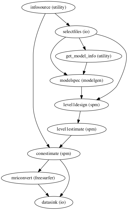
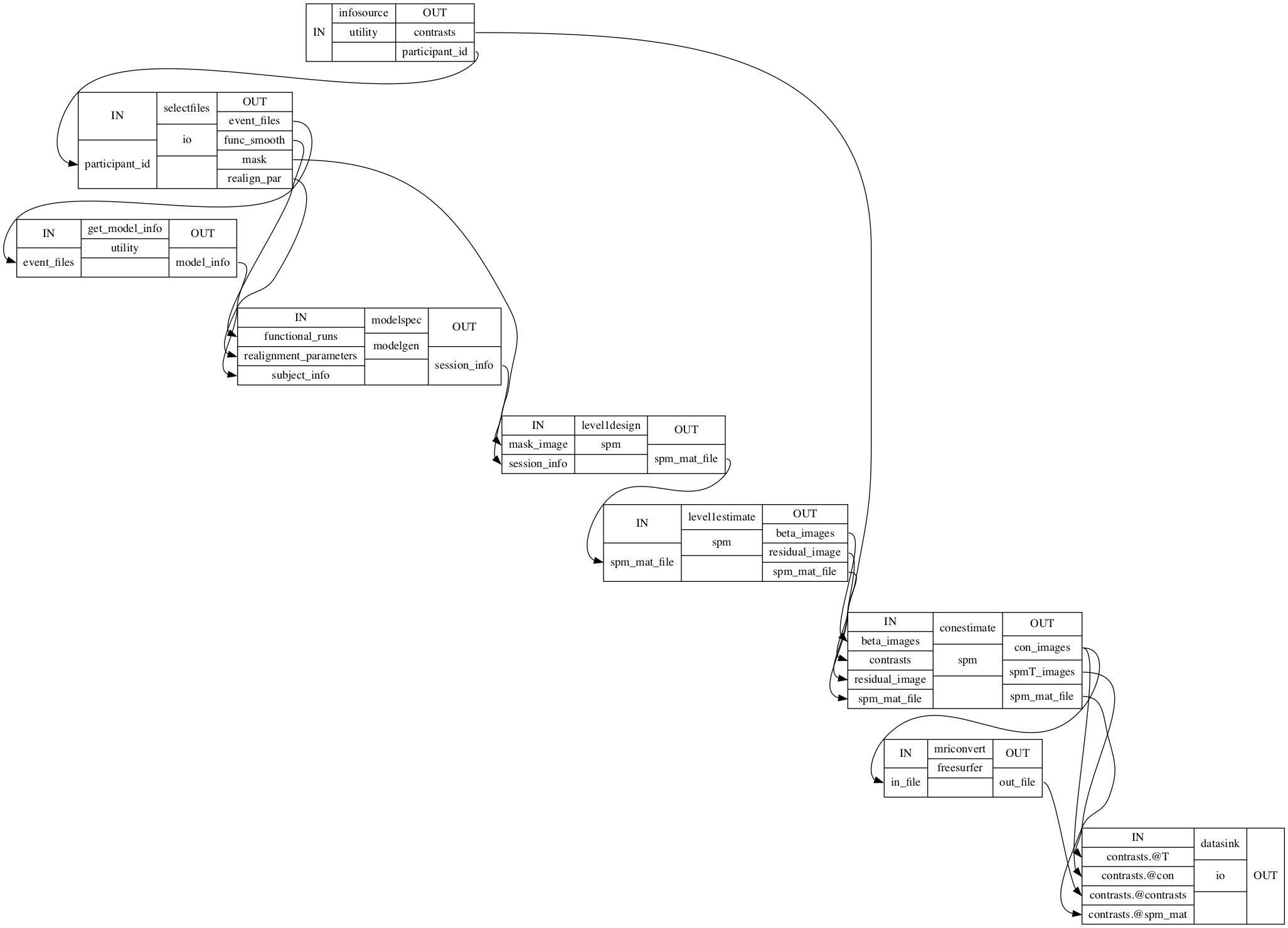
Evaluate the workflow
As done during preprocessing, we will evaluate our workflow by generating graphs that visualize the inputs and outputs of our nodes.
ind_level.write_graph(graph2use='colored',format='png', simple_form=True)


ind_level.write_graph(graph2use='flat',format='png', simple_form=True)
'/data/mvs/derivatives/individual_level/workingdir_individual_statistics/ind_level/graph.png'
Let’s check them:
from IPython.display import Image
Image(filename="/data/mvs/derivatives/individual_level/workingdir_individual_statistics/ind_level/graph.png")
Image('/data/mvs/derivatives/individual_level/workingdir_individual_statistics/ind_level/graph_detailed.png')
Native space - template space registration
As usual, let’s important necessary modules and functions before we start.
Import Modules
from nipype.interfaces.ants import Registration
from nipype.interfaces.fsl import Info
Define and set important paths
You know the drill, new processing stage, new output and working directory path.
output_dir = 'derivatives/registration'
working_dir = 'derivatives/registration/workingdir'
Define and set processing nodes
Now that we have our contrast images that contain the cortical responses evoked through our stimuli, we can start the process of bringing them in a shared template space. For the majority of group level analyses, this is a necessity and even though we won’t do a “classic” mass-univariate group level analyses, we still need it for the planned MVPA. We want to achieve the transformation from native functional to template space via a two-step procedure: native functional -> native anatomical -> template. As we have contrast images in a given participants native space and already computed the coregistration between functional and anatomical space for each participant, we’re only missing the coregistration between a given participants native anatomical space and the template space. We’re going to use the fantastic ANTs software for that, more specifically it’s Registration function.
antsreg = Node(Registration(args='--float',
                            collapse_output_transforms=True,
                            fixed_image=template,
                            initial_moving_transform_com=True,
                            num_threads=1,
                            output_inverse_warped_image=True,
                            output_warped_image=True,
                            sigma_units=['vox']*3,
                            transforms=['Rigid', 'Affine', 'SyN'],
                            terminal_output='file',
                            winsorize_lower_quantile=0.005,
                            winsorize_upper_quantile=0.995,
                            convergence_threshold=[1e-06],
                            convergence_window_size=[10],
                            metric=['MI', 'MI', 'CC'],
                            metric_weight=[1.0]*3,
                            number_of_iterations=[[1000, 500, 250, 100],
                                                  [1000, 500, 250, 100],
                                                  [100, 70, 50, 20]],
                            radius_or_number_of_bins=[32, 32, 4],
                            sampling_percentage=[0.25, 0.25, 1],
                            sampling_strategy=['Regular',
                                               'Regular',
                                               'None'],
                            shrink_factors=[[8, 4, 2, 1]]*3,
                            smoothing_sigmas=[[3, 2, 1, 0]]*3,
                            transform_parameters=[(0.1,),
                                                  (0.1,),
                                                  (0.1, 3.0, 0.0)],
                            use_histogram_matching=True,
                            write_composite_transform=True),
               name='antsreg')
We decided to go with the MNI152 template in its non-linear symmetric version given its frequent and established usage, particularly its support in other higher level toolboxes/resources (e.g. neuorsynth). Through nipype’s FSL interface, i.e. the Info function, we can easily gather the template.
template = Info.standard_image('MNI152_T1_1mm_brain.nii.gz')
And check it out using nilearn (it’s interactive, you can scroll through the template image!).
from nilearn.plotting import view_img
view_img(template, cmap='Greys', draw_cross=False, colorbar=False, dim=-2)
Fancy, let’s set it as fixed_image within our Registration node, that is defining it as the image the moving image (anatomical image) should be coregistered to.
antsreg.inputs.fixed_image=template
Create the workflow and connect the nodes
As this is basically a one processing node workflow we can already create the empty workflow and set input and output streams. First things first, the workflow.
coreg_ANTs = Workflow(name='coreg_ANTs')
coreg_ANTs.base_dir = opj(experiment_dir, working_dir)
Hello IdentityInterface funcion my old friend…
infosource = Node(IdentityInterface(fields=['participant_id']),
                  name="infosource")
infosource.iterables = [('participant_id', participant_list)]
Given that the template is already defined, we only need to provide the path for the anatomical images within the templat paths of the SelectFiles function.
templates = {'anat': '/data/mvs/derivatives/mindboggle/freesurfer/{subject_id}/mri/brain.mgz',
             }

selectfiles = Node(SelectFiles(templates,
                               base_directory=experiment_dir),
                   name="selectfiles")
The output is handled by the DataSink function again.
datasink = Node(DataSink(base_directory=experiment_dir,
                         container=output_dir),
                name="datasink")
No DataSink without substitutions.
substitutions = [('_participant_id_', '')]
datasink.inputs.substitutions = substitutions
Connecting the nodes is done in no time for this processing stage:
coreg_ANTs.connect([(infosource, selectfiles, [('participant_id', 'participant_id')]), # select files from participants
                    (selectfiles, antsreg, [('anat', 'moving_image')]), # set anatomical image as moving image
                    (antsreg, datasink, [('warped_image', 'antsreg.@warped_image'), # send transformed image to datasink
                                         ('inverse_warped_image', 'antsreg.@inverse_warped_image'), # send inverse transformed image to datasink
                                         ('composite_transform', 'antsreg.@transform'), # send transformation matrices to datasink
                                         ('inverse_composite_transform', 'antsreg.@inverse_transform')]), # send inverse transformation matrices to datasink
                  ])
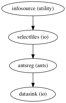
Evaluate the workflow
Using the same functions as for the preprocessing and individual level statistics we can visualize the workflow:
coreg_ANTs.write_graph(graph2use='colored',format='png', simple_form=True)


coreg_ANTs.write_graph(graph2use='flat',format='png', simple_form=True)
'/data/mvs/derivatives/registration/workingdir/coreg_ANTs/graph.png'
from IPython.display import Image
Image(filename="/data/mvs/derivatives/registration/workingdir/coreg_ANTs/graph.png")
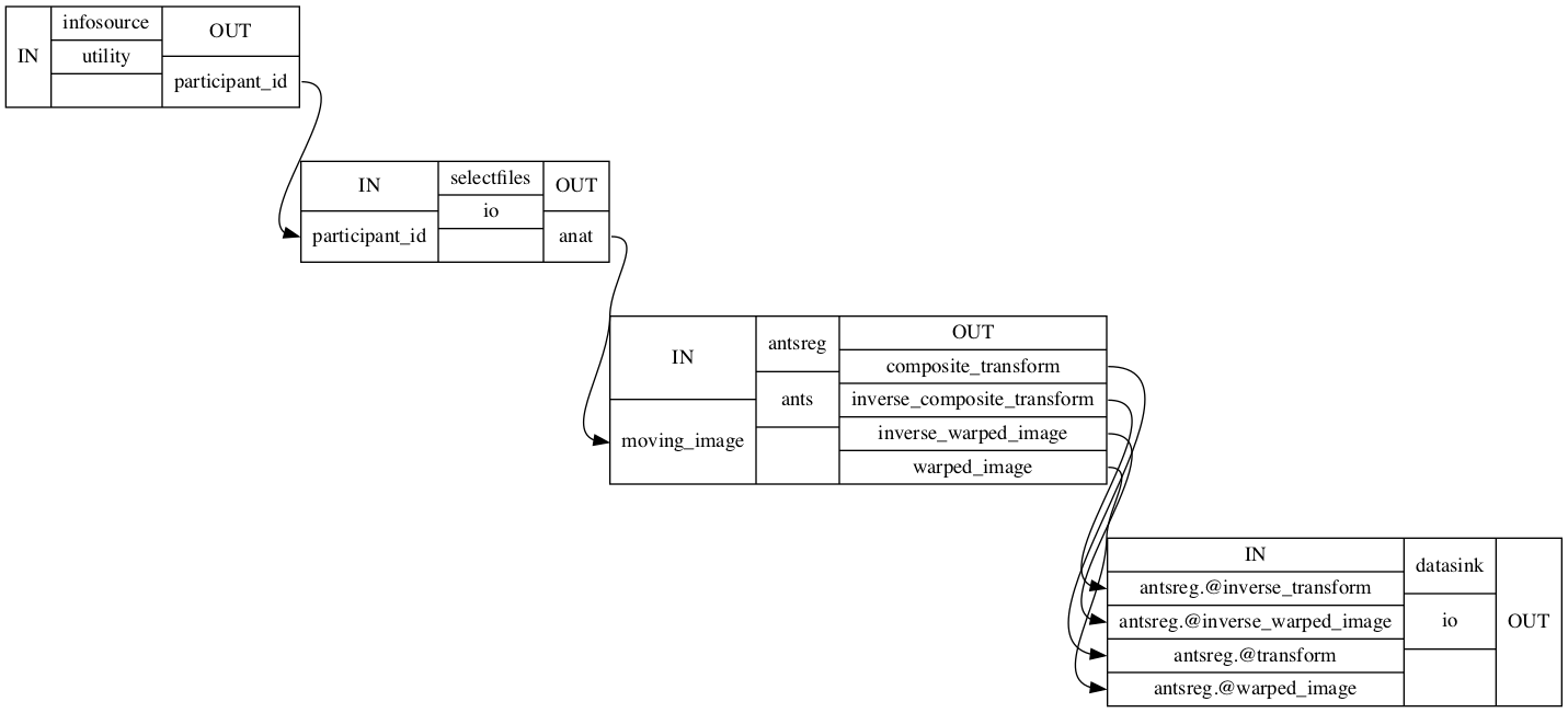
Image(filename="/data/mvs/derivatives/registration/workingdir/coreg_ANTs/graph_detailed.png")
Native space to template space transformation
Now that we have our contrast images in participant specific functional space that contain the cortical responses evoked through our stimuli, we can start the process of bringing them in a shared template space. For the majority of group level analyses, this is a necessity and even though we won’t do a “classic” mass-univariate group level analyses, we still need it for the planned MVPA. We want to achieve the transformation from native functional to template space via a two-step procedure: native functional -> native anatomical -> template. As we have contrast images in a given participants native space and already computed the coregistration between functional and anatomical space, as well as snatomical and template space for each participant, we only need to concatenate the respective transformation matrices and apply them to the images. As we want to use ANTs for the transformation, we need to convert the transformation matrix obtained through bbregister to ITK format. We’ll do this via the C3DAffineTool.
Import modules
Let’s import the modules and functions we need for this step.
from nipype.interfaces.ants import ApplyTransforms
from nipype.interfaces.c3 import C3dAffineTool
from nipype.interfaces.utility.base import Merge
Define and set important paths and variables
As we need a few files from previous processing steps, we set a set of paths, including the preprocessing, individual level statistics and registration folders.
input_dir_individual_level = '/data/mvs/derivatives/individual_level'
input_dir_reg = '/data/mvs/derivatives/registration'
input_dir_preproc = '/data/mvs/derivatives/preprocessing'
The output and working directory are defined as usual.
output_dir = '/data/mvs/derivatives/transformation_functional'
working_dir = '/data/derivatives/transformation_functional/workingdir'
Define and set processing nodes
As outlined above, some steps are needed to achieve our goal. More precisely, we need the C3DAffineTool, Nipype’s Merge function and ANTs’ ApplyTransforms function. The first is necessary, as ANTs likes the ITK format and thus we need to convert the FSL registration file obtained during the coregistration step of the preprocessing accordingly. To do so, the function needs all inputs of the original coregistration function, as well as the computed registration matrix. Those parts will be set within the workflow. Here we’ll only create the node and set conversion specific information, i.e. that an FSL registration matrix will be used and that we want to obtain an ITK format.
convert2itk = Node(C3dAffineTool(fsl2ras=True,
                                 itk_transform=True),
                   name='convert2itk')
In order to avoid multiple transformations of the same image, we want to concatenate our registration matrices (from functional to anatomical space and from anatomical to template space. That’s easily done using Nipype’s Merge function. We indicate that we want to concatenate 2 inputs into one list.
merge = Node(Merge(2), name='merge')
Now to the actual transformation which we will be running through ANTs’ ApplyTransforms function. Comparably to the registration, ANTs is more complex than other software packages (which IMHO is a good thing). There are a lot of input parameters we can set, so let’s go through them step by step. Starting easy, our reference image is already set through the same template we used during the anatomical to template space coregistration. Through args=='--float' we indicate that we want to use floats instead of double for computation. We set input_image_type to 3 as we don’t have vector or tensor, but time series images. Next, we define a linear interpolation and that we don’t want to invert our transformation matrices. To not stress our machine too much, we will run the transformation on 1 thread. Finally, as we want to transform multiple images, we set the input_image as an interfield.
warpall = MapNode(ApplyTransforms(args='--float',
                                  input_image_type=3,
                                  interpolation='Linear',
                                  invert_transform_flags=[False, False],
                                  num_threads=1,
                                  reference_image=template,
                                  terminal_output='file'),
                  name='warpall', iterfield=['input_image'])
We are also going to transform the mean functional image as a sanity check via defining the same node as before, but with a different name.
warpmean = Node(ApplyTransforms(args='--float',
                                input_image_type=3,
                                interpolation='Linear',
                                invert_transform_flags=[False, False],
                                num_threads=1,
                                reference_image=template,
                                terminal_output='file'),
                name='warpmean')
Create the workflow and connect the nodes
With all processing nodes set, we can create our transformation workflow and connect the nodes. The classic: the workflow first.
norm_ANTS_flow = Workflow(name='norm_ANTS_flow')
norm_ANTS_flow.base_dir = opj(experiment_dir, working_dir)
And now to the nodes. Please note, that we only need to connect the merge and transformation nodes at this point, as the other nodes will be connected within the input streams.
norm_ANTS_flow.connect([(merge, warpmean, [('out', 'transforms')]), # provide concatenated transformation matrices for contrast image transformation
                        (merge, warpall, [('out', 'transforms')]), # provide concatenated transformation matrices for mean functional image transformation
                      ])
The IdentityInterface is back once more to help us define our input stream and as before we set the participant_list as input to iterate over.
infosource = Node(IdentityInterface(fields=['participant_id']),
                  name="infosource")
infosource.iterables = [('participant_id', participant_list)]
Now to the templates for the SelectFiles function. As mentioned above, we need a few for this step: the mean functional image from the realignment step of the preporcessing, the skull-stripped anatomical image from the FreeSurfer recon-all pipeline within the structural preprocessing step, the registration matrix from the coregistration step of the preprocessing, the registration matrix from the anatomical to template registration and the contrast images from the individual level statistical analyses.
templates = {'reg_file' : opj(input_dir_reg, 'bbregister', '{subject_id}', 'mean*.mat'),
             'transform_composite' : opj(input_dir_reg, 'antsreg', '{subject_id}', 'transformComposite.h5'),
             'func_orig': opj(input_dir_individual_level, 'contrasts','{subject_id}', 'con*.nii'),
             'anat': '/data/mvs/derivatives/mindboggle/freesurfer/{subject_id}/mri/brain.mgz',
             'mean': opj(input_dir_preproc, 'realign', '{subject_id}', 'mean*.nii'),
             }
And the SelectFiles function itself, with the defined templates and the experiment directory as base directory.
selectfiles = Node(SelectFiles(templates,
                               base_directory=experiment_dir),
                   name="selectfiles")
Identical to the other processing steps, we will use DataSink to set our output streams and define substitutions.
datasink = Node(DataSink(base_directory=experiment_dir,
                         container=output_dir),
                name="datasink")

substitutions = [('_subject_id_', ''),
                 ('_apply2con', ''),
                 ('_warpall', '')]
datasink.inputs.substitutions = substitutions
Ready, set, connect nodes.
norm_ANTS_flow.connect([(infosource, selectfiles, [('participant_id', 'participant_id')]), # select files from participants
                        (selectfiles, convert2itk, [('anat', 'reference_file')]), # set anatomical image as reference file
                        (selectfiles, convert2itk, [('mean', 'source_file')]), # set mean functional image as source file
                        (selectfiles, convert2itk, [('reg_file', 'transform_file')]), # set registration file as transform file
                        (convert2itk, merge, [('itk_transform', 'in1')]), # set transformation matrix in ITK format (function to anatomical) as first transformation
                        (selectfiles, merge, [('transform_composite', 'in2')]), # set ants tranformation matrix (anatomical to template) as second transformation
                        (selectfiles, warpall, [('func_orig', 'input_image')]), # transform contrast images to template space
                        (selectfiles, warpmean, [('mean', 'input_image')]), # transform mean functional image to template space
                        (warpall, datasink, [('output_image', 'warp_complete.@warpall')]), # send transformed contrast images to datasink
                        (warpmean, datasink, [('output_image', 'warp_complete.@warpmean')]), # send transformed mean functional image to datasink
                      ])
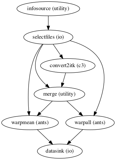
For the last time in this overarching processing step, we’re going to evaluate the workflow by visualizing it in two ways: a simple and a detailed graph.
norm_ANTS_flow.write_graph(graph2use='colored',format='png', simple_form=True)

norm_ANTS_flow.write_graph(graph2use='flat',format='png', simple_form=True)
'/data/mvs/derivatives/transformation_functional/workingdir/norm_ANTS_flow/graph.png'
from IPython.display import Image
Image(filename="/data/mvs/derivatives/transformation_functional/workingdir/norm_ANTS_flow/graph.png")
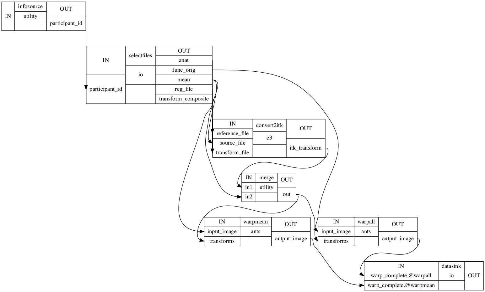
Image(filename="/data/mvs/derivatives/transformation_functional/workingdir/norm_ANTS_flow/graph_detailed.png")
Summary and outlook
Well, that was quite a ride, eh? As a lot happened since we started, let’s briefly summarize everything and peak into what follows. The above processing steps and corresponding code/workflows depict the conducted analyses, including structural and functional preprocessing, individual level statistics, native to template space registration and native to template space transformation. Everything was implemented in nipype workflows and throughout the steps we used a broad range of software packages consisting of SPM, FSL, FreeSurfer and ANTs. Our goal was to prepare the acquired data for subsequent analyses, especially MVPA. The outcomes of the steps shown here were further employed in other steps of our analysis and are referred to respectively. Please note, that we conducted a different individual level statistical analyses within the connectivity analyses as we needed a different model. The next section will be provide details on the utilized auditory cortex model.