Searchlight and ROI decoding
Within the following, the conducted MVPA, that is searchlight and ROI decoding analyses, are shown, explained and set up in way that they can be rerun and the results be reproduced. It is divided into the following sections:
Prerequisites
create label and subject list for cross-validation
set important files
defining analysis parameters - feature scaling & classifier
defining analysis parameters - cross-validation
defining analysis parameters - permutation test
defining analysis parameters - connecting the dots
Searchlight analyses
multiclass
music vs. singing
music vs. speech
singing vs. speech
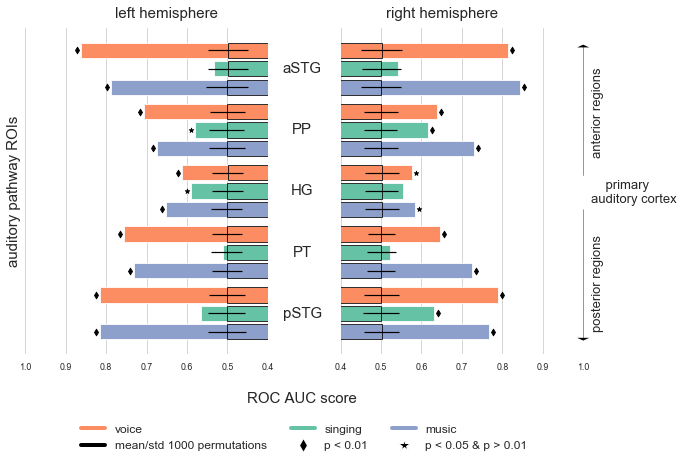
ROI decoding analyses
multiclass
music vs. singing
music vs. speech
singing vs. speech
single condition decoding
We provide more detailed information and explanations in the respective sections. As mentioned before, we’re working with derivatives here and thus we can share them, meaning that you can rerun the analyses either by downloading this page as a Jupyter Notebook (via the download button at the top) or interactively via a cloud instance through the amazing mybinder project (the little rocket at the top). We recommend the later to spare installation and conda environment related problems. One more thing… Please note, that derivatives refer to the contrast images we computed in the previous sections which we provide via the project’s OSF page because their computation is computationally very expensive and would never run via the resources available through binder. However, we included the code and explanations depicting how this steps were run. The code that will download the required data is included in the respective sections. Some of the processes here are computationally expensive and thus might take a while to run. If you don’t want to/can’t do that or just want to get the data: we provide the searchlight maps and ROI decoding results via different means. The first can be accessed via a neurovault collection and both through the OSF project. Whenever possible we provide this option through corresponding code that will download the data, if you choose to do so.
Before we start, we need to import the packages and functions we are going to use.
Import modules
As usual, the first thing we do is to import modules and functions we are going to use throughout the analyses. As you can see there are quite a bunch of them. However, we are also going to run quite a bunch of analyses, thus it’s fair.
from glob import glob
import os
from os.path import join as opj
import json
import nibabel as nb
from nilearn.image import math_img, new_img_like, index_img, threshold_img, get_data
from nilearn.plotting import plot_img
import pandas as pd
import seaborn as sns
import ptitprince as pt
from sklearn.model_selection import GroupShuffleSplit, cross_val_score, permutation_test_score
from sklearn.multiclass import OneVsRestClassifier
from sklearn.metrics import auc, plot_roc_curve
from nilearn.decoding import SearchLight
from nilearn.input_data import NiftiMasker
from nilearn.datasets import load_mni152_template
from nilearn.plotting import plot_roi, plot_anat, view_img, view_img_on_surf
from sklearn.svm import SVC
from sklearn.pipeline import make_pipeline
from sklearn.preprocessing import StandardScaler
from sklearn.dummy import DummyClassifier
from sklearn import clone
import numpy as np
import scipy.stats as st
import matplotlib.pyplot as plt
from matplotlib.lines import Line2D
from matplotlib import colors
%matplotlib inline
Let’s also gather and set some important paths. This includes the path to the general derivatives directory, as well as analyses specific ones. In more detail, we of course aim to keep it as BIDS-y as possible and therefore set a new path for the MVPA run here. To keep results and necessary prerequisites separate (keeping it tidy), we also create a dedicated directory which will include the participant/label information, as well as the input data.
derivatives_path = '/data/mvs/derivatives/'
roi_mask_path ='/data/mvs/derivatives/ROIs_masks/'
individual_level ='/data/mvs/derivatives/individual_level/warp_complete/'
prereq_path = '/data/mvs/derivatives/MVPA/prerequisites/'
results_path = '/data/mvs/derivatives/MVPA/'
Prerequisites
At first, we need to define and set some important prerequisites that we will need throughout the analyses. This includes a participant and label list that we will use for the applied cross-validation, as well as the image files and data on which we will perform the analyses.
create label and subject list for cross-validation
For the intended cross-validation, we need to generate lists that will allow us to indicate to which participant and label (or category) a certain piece of data belongs to. This is important and necessary to define training and test sets, as well as classification tasks. We have three categories (music, singing, voice) for each of 24 participants. Please note, that we exclude sub-06 from our analyses as this participant didn’t show reliable responses at the individual level. In order to have everything nicely organized, we will put our generated participant and category list into a pandas dataframe and save it within the set derivatives/MVPA/prerequisites path.
labels = list(('music', 'singing', 'voice')*23)
participants = []
for part in range(1,25):
if part == 6:
continue
elif part < 10:
participants.append('sub-0%s' % str(part))
participants.append('sub-0%s' % str(part))
participants.append('sub-0%s' % str(part))
elif part >= 10:
participants.append('sub-%s' % str(part))
participants.append('sub-%s' % str(part))
participants.append('sub-%s' % str(part))
decoding_info = pd.DataFrame({'labels':labels, 'participants':participants})
decoding_info.to_csv(opj(prereq_path,'decoding_info.csv'), index = False)
Let’s check what we have in decoding_info:
decoding_info
| labels | participants | |
|---|---|---|
| 0 | music | sub-01 |
| 1 | singing | sub-01 |
| 2 | voice | sub-01 |
| 3 | music | sub-02 |
| 4 | singing | sub-02 |
| 5 | voice | sub-02 |
| 6 | music | sub-03 |
| 7 | singing | sub-03 |
| 8 | voice | sub-03 |
| 9 | music | sub-04 |
| 10 | singing | sub-04 |
| 11 | voice | sub-04 |
| 12 | music | sub-05 |
| 13 | singing | sub-05 |
| 14 | voice | sub-05 |
| 15 | music | sub-07 |
| 16 | singing | sub-07 |
| 17 | voice | sub-07 |
| 18 | music | sub-08 |
| 19 | singing | sub-08 |
| 20 | voice | sub-08 |
| 21 | music | sub-09 |
| 22 | singing | sub-09 |
| 23 | voice | sub-09 |
| 24 | music | sub-10 |
| 25 | singing | sub-10 |
| 26 | voice | sub-10 |
| 27 | music | sub-11 |
| 28 | singing | sub-11 |
| 29 | voice | sub-11 |
| ... | ... | ... |
| 39 | music | sub-15 |
| 40 | singing | sub-15 |
| 41 | voice | sub-15 |
| 42 | music | sub-16 |
| 43 | singing | sub-16 |
| 44 | voice | sub-16 |
| 45 | music | sub-17 |
| 46 | singing | sub-17 |
| 47 | voice | sub-17 |
| 48 | music | sub-18 |
| 49 | singing | sub-18 |
| 50 | voice | sub-18 |
| 51 | music | sub-19 |
| 52 | singing | sub-19 |
| 53 | voice | sub-19 |
| 54 | music | sub-20 |
| 55 | singing | sub-20 |
| 56 | voice | sub-20 |
| 57 | music | sub-21 |
| 58 | singing | sub-21 |
| 59 | voice | sub-21 |
| 60 | music | sub-22 |
| 61 | singing | sub-22 |
| 62 | voice | sub-22 |
| 63 | music | sub-23 |
| 64 | singing | sub-23 |
| 65 | voice | sub-23 |
| 66 | music | sub-24 |
| 67 | singing | sub-24 |
| 68 | voice | sub-24 |
69 rows × 2 columns
Looks ok, we have 69 rows, i.e. 23 participants * 3 categories. As we saved it to the dedicated path, we can move on to the next step.
Set important files and objects
There are a few important files and objects we are going to need throughout the analyses. This includes the auditory cortex mask we created in the previous step, the contrast images we computed in the individual level statistics and the image data we extract from the contrast images using the auditory cortex mask. Speaking of which, let’s check our mask again. At first, we are going to set the respective path
ac_mask = opj(roi_mask_path, 'tpl-MNI152NLin6Sym_res_02_desc-ACdilated_mask.nii.gz')
and then plot it on the MNI152 template image.
fig=plt.figure(num=None, figsize=(12, 6))
check_ROIs = plot_anat(cut_coords=[-60, -34, 7], figure=fig, draw_cross=False)
check_ROIs.add_contours(ac_mask,
levels=[0], colors='black')
plt.text(-230, 90, 'Auditory cortex mask',
fontsize=22)
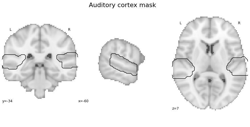
Next, we create a nilearn NiftiMasker object indicating the auditory cortex mask as mask image in order to be able to extract voxel patterns that fell within this mask. Please remember that we created this mask in the previous step specifically to restrict our analyses to the auditory cortex, as we were focusing on its functional principles.
ac_masker = NiftiMasker(mask_img=ac_mask, memory="nilearn_cache", memory_level=1)
So far so good. What’s missing is a crucial part: the data we want to analyze. As outlined before, we’re going to use the contrast images we computed within the preprocessing & individual level statistics section. This in particular refers to the category specific contrast images estimated across both runs transformed to the template space. Thus, we will have three contrast images (one for each category: music, singing and voice) per participant. Originally, these were gathered and concatenated to a 4D image to have everything needed nicely in place and allow easy sharing. This was conducted via nibabel:
list_con_images = []
for part in range(1,25):
for con in range(7,10):
if part == 6:
continue
elif part < 10:
list_cons.append(opj(individual_level, 'sub-0%s' %str(part), 'con_000%s.nii.gz' %str(con)))
elif part >= 10:
list_cons.append(opj(individual_level, 'sub-%s' %str(part), 'con_000%s.nii.gz' %str(con)))
con_images_concat = nb.concat_images(list_con)
con_images_concat.to_filename(opj(prereq_path,'task-mvs_space-MNI152NLin6Sym_desc-con.nii.gz'))
We provide the resulting image in the project’s OSF page and thus can download it through the OSF client. It’s a command line thingy for which we have to indicate the OSF project ID (-p) and from where (in the OSF repository) to where ( on our local machine) we want to fetch it.
osf -p <projectid> fetch remote/path.txt local/file.txt
Having downloaded the requiered file, we can set it accordingly for further analyses.
con_images = opj(prereq_path, 'task-mvs_space-MNI152NLin6Sym_desc-con.nii.gz')
Great! However, as some planned analyses have to be run on the extracted data and not the contrast images, we’ll also already extract the data from the contrast images. As outlined multiple times before, we want to restrict our analyses to the auditory cortex and thus can fit the NiftiMasker we set a few steps before:
con_images_data = ac_masker.fit_transform(con_images)
Let’s check what we have in con_images_data now, as well as it’s dimensions:
con_images_data
array([[ 4.2127714e-01, 9.5591199e-01, 1.4899406e+00, ...,
1.1660988e+00, 1.7181042e+00, 2.5876074e+00],
[ 4.5708263e-01, 1.0267698e+00, 1.4634324e+00, ...,
1.5170587e+00, 2.5045147e+00, 3.4200864e+00],
[ 2.5726053e-01, 7.2290897e-01, 9.8951960e-01, ...,
2.8223815e+00, 4.4414096e+00, 5.9877033e+00],
...,
[ 2.6815426e-01, 2.4177605e-01, -1.8233545e-01, ...,
1.1213929e-01, 9.4061546e-02, 3.9933190e-18],
[-4.9079783e-02, -4.7520988e-02, -3.9716083e-01, ...,
2.5803149e-01, 2.0084761e-01, 8.5735730e-19],
[-5.1823610e-01, -5.3660983e-01, -5.4666173e-01, ...,
3.1283933e-01, 2.3260626e-01, 1.4010841e-17]], dtype=float32)
con_images_data.shape
(69, 9652)
As you can see, we have an array of the dimensions 69 by 9652 containing numerical values. In more detail, we have the data of voxels (the array) that fell within the auditory cortex mask (9652) from each of three contrast images of 23 participants (3 x 23 = 69). It appears that everything fits and the necessary information and data set. Thus, we can continue with the next part of the prerequisites, the analyses parameters.
Analysis parameters
As you might have heard: machine learning analyses are incredibly complicated and, if applied without care, can lead to substaintially misleading results and thus conclusions. The analyses conducted here are no exception to that. And while there are no definite “this-is-how-you-do-it” guidelines, there are however guidelines that, based on simulated and real data, provide certain recommendations and “no-gos” [REF]. We’ll discuss this in the following section and accordingly set up the general and important parameters of the analyses: feature scaling, classifier, cross-validation and permutations. Importantly, the corresponding parameters were identical across both, the searchlight and ROI decoding analyses. At first, let’s load the decoding_info.csv file we specified above and which includes information necessary with regard to the CV and task itself: the labels (aka conditions) and participants.
decoding_info = pd.read_csv(opj(prereq_path,'decoding_info.csv'), sep=',')
conditions = decoding_info['labels']
participants = decoding_info['participants']
print(decoding_info)
print(decoding_info['labels'].unique())
print(decoding_info['participants'].unique())
labels participants
0 music sub-01
1 singing sub-01
2 voice sub-01
3 music sub-02
4 singing sub-02
.. ... ...
64 singing sub-23
65 voice sub-23
66 music sub-24
67 singing sub-24
68 voice sub-24
[69 rows x 2 columns]
['music' 'singing' 'voice']
['sub-01' 'sub-02' 'sub-03' 'sub-04' 'sub-05' 'sub-07' 'sub-08' 'sub-09'
'sub-10' 'sub-11' 'sub-12' 'sub-13' 'sub-14' 'sub-15' 'sub-16' 'sub-17'
'sub-18' 'sub-19' 'sub-20' 'sub-21' 'sub-22' 'sub-23' 'sub-24']
That looks about right. Hence, we continue with the parameters of our analyses, starting with feature scaling and the classifier.
Defining the analyses parameters: feature scaling and classifier
For folks experienced with machine learning it’s no secret that, before running the planned analyses, the features which enter should be scaled (for a quick explanation and motivation check the corresponding wikipedia site). Within the analyses at hand, the features are the voxel patterns and the voxel reponses within them, associated with/evoked by the different conditions (music, singing, speech) as assesed by the 1st level analyses and reflected in the contrast images we’re utilizing here. There are different ways to do feature scaling, with varying results. Two common approaches are the MinMaxScaler and the StandardScaler (here as implemented in scikit-learn). Here, we’re going to use the later, thus scaling “… by removing the mean and to unit variance” (scikit-learn docs section on StandardScaler).
The next crucial thing is the classifier, that is the algorithm that implements the classification. Comparable to feature scaling, the choice of the classifier is one of the many knobes to turn within a machine learning analysis that can heavily influence the obtained results and thus interpretation. Again, there’s a vast variety to choose from (e.g. list of supervised classifiers in scikit-learn and classifier comparison in the scikit-learn docs) and the “right” classifier is not always obvious or existent as it depends on the data, task, etc. (for some reviews, overview pieces, etc. please have a look here, here, here, here and here). Given the dimensionality and nature of the data, together with no strong assumptions regarding the distribution, a linear classifier such as a linear support vector machine (SVM) might be a good starting point. Here we’re going to use scikit-learn’s implementation of C-Support Vector classification with the default regularization paramter of C = 1 and a linear kernel.
When it comes to implementing these things were are lucky. Instead of applying/setting these things in a stepwise manner, we can make use of scikit-learn’s make_pipeline function and just create a pipeline within which we set the succession of StandardScaler and SVC.
pipeline = make_pipeline(StandardScaler(), SVC(kernel='linear'))
With these things set, we can continue to the next analyses parameter: cross-validation.
defining analysis parameters - cross-validation
Another central aspect of any machine learning analysis is cross-validation (CV). The basic idea is that we split our data in different partitions, sets or folds, one to train our classifier and one to test it on (ideally there would also be a validation partition as well). In neuroimaging CV is quite often implement based on runs within an experiment and utilizing a so called leave-one-out CV. Assuming you have 5 runs you would train your classifier on the data from 4 runs and test it on the data from the remaining run. You would then repeat this procedure until each run was the test set once. However, in this project we applied a different CV based on two reasons. First, prior research on real and simulated data [REF] has shown that other CV types should be preferred over leave-one-out. Second, a sufficient within-participant CV based on a leave-one-out CV was not possible given the utilized paradigm constituted an event-related paradigm within which three conditions (our sound categories) were presented in two runs. Thus, each run could only serve as train and test set once. To address this problem, we used a between participant CV, that is we trained a the classifier on the data from a subset of participant and tested it on the data from the remaining participants. In more detail, a GroupShuffleSplit CV with 10 splits and a training size of 0.8 was set up. We choose this CV as it allows to conduct a repeated k-fold CV within which a group parameter can be defined in order to indicate restrictions of how the data should be splitted. In our case, we needed to make sure that a given participant is only part of the training or test set, but not both. The outcome of the classification task per fold is then averaged across to obtain a final evaluation. Let’s setup and evaluate our CV. At first, we need define it as mentioned above (please note that we are also setting the random state to make splits reproducible).
cv = GroupShuffleSplit(n_splits=10, train_size=.8, random_state=42)
Now, we can apply this CV to our data and evaluate the resulting train and test sets per fold. To this end, we need to provide our con_image_data, the condition labels and the groups parameter. Both, the condition labels and participant labels (used to define groups) are available through the decoding_info dataframe and were already set a few steps prior.
for train, test in cv.split(con_images_data, conditions, groups=participants):
print("training classifier on: \n",
participants.to_numpy()[train],
"\n",
conditions.to_numpy()[train],
"\n",
"testing classifier on: \n",
participants.to_numpy()[test],
"\n",
conditions.to_numpy()[test])
training classifier on:
['sub-02' 'sub-02' 'sub-02' 'sub-03' 'sub-03' 'sub-03' 'sub-04' 'sub-04'
'sub-04' 'sub-05' 'sub-05' 'sub-05' 'sub-07' 'sub-07' 'sub-07' 'sub-08'
'sub-08' 'sub-08' 'sub-09' 'sub-09' 'sub-09' 'sub-12' 'sub-12' 'sub-12'
'sub-13' 'sub-13' 'sub-13' 'sub-14' 'sub-14' 'sub-14' 'sub-15' 'sub-15'
'sub-15' 'sub-16' 'sub-16' 'sub-16' 'sub-18' 'sub-18' 'sub-18' 'sub-20'
'sub-20' 'sub-20' 'sub-21' 'sub-21' 'sub-21' 'sub-22' 'sub-22' 'sub-22'
'sub-23' 'sub-23' 'sub-23' 'sub-24' 'sub-24' 'sub-24']
['music' 'singing' 'voice' 'music' 'singing' 'voice' 'music' 'singing'
'voice' 'music' 'singing' 'voice' 'music' 'singing' 'voice' 'music'
'singing' 'voice' 'music' 'singing' 'voice' 'music' 'singing' 'voice'
'music' 'singing' 'voice' 'music' 'singing' 'voice' 'music' 'singing'
'voice' 'music' 'singing' 'voice' 'music' 'singing' 'voice' 'music'
'singing' 'voice' 'music' 'singing' 'voice' 'music' 'singing' 'voice'
'music' 'singing' 'voice' 'music' 'singing' 'voice']
testing classifier on:
['sub-01' 'sub-01' 'sub-01' 'sub-10' 'sub-10' 'sub-10' 'sub-11' 'sub-11'
'sub-11' 'sub-17' 'sub-17' 'sub-17' 'sub-19' 'sub-19' 'sub-19']
['music' 'singing' 'voice' 'music' 'singing' 'voice' 'music' 'singing'
'voice' 'music' 'singing' 'voice' 'music' 'singing' 'voice']
training classifier on:
['sub-03' 'sub-03' 'sub-03' 'sub-04' 'sub-04' 'sub-04' 'sub-05' 'sub-05'
'sub-05' 'sub-08' 'sub-08' 'sub-08' 'sub-09' 'sub-09' 'sub-09' 'sub-10'
'sub-10' 'sub-10' 'sub-11' 'sub-11' 'sub-11' 'sub-13' 'sub-13' 'sub-13'
'sub-14' 'sub-14' 'sub-14' 'sub-15' 'sub-15' 'sub-15' 'sub-16' 'sub-16'
'sub-16' 'sub-17' 'sub-17' 'sub-17' 'sub-18' 'sub-18' 'sub-18' 'sub-19'
'sub-19' 'sub-19' 'sub-21' 'sub-21' 'sub-21' 'sub-22' 'sub-22' 'sub-22'
'sub-23' 'sub-23' 'sub-23' 'sub-24' 'sub-24' 'sub-24']
['music' 'singing' 'voice' 'music' 'singing' 'voice' 'music' 'singing'
'voice' 'music' 'singing' 'voice' 'music' 'singing' 'voice' 'music'
'singing' 'voice' 'music' 'singing' 'voice' 'music' 'singing' 'voice'
'music' 'singing' 'voice' 'music' 'singing' 'voice' 'music' 'singing'
'voice' 'music' 'singing' 'voice' 'music' 'singing' 'voice' 'music'
'singing' 'voice' 'music' 'singing' 'voice' 'music' 'singing' 'voice'
'music' 'singing' 'voice' 'music' 'singing' 'voice']
testing classifier on:
['sub-01' 'sub-01' 'sub-01' 'sub-02' 'sub-02' 'sub-02' 'sub-07' 'sub-07'
'sub-07' 'sub-12' 'sub-12' 'sub-12' 'sub-20' 'sub-20' 'sub-20']
['music' 'singing' 'voice' 'music' 'singing' 'voice' 'music' 'singing'
'voice' 'music' 'singing' 'voice' 'music' 'singing' 'voice']
training classifier on:
['sub-01' 'sub-01' 'sub-01' 'sub-02' 'sub-02' 'sub-02' 'sub-03' 'sub-03'
'sub-03' 'sub-04' 'sub-04' 'sub-04' 'sub-07' 'sub-07' 'sub-07' 'sub-08'
'sub-08' 'sub-08' 'sub-09' 'sub-09' 'sub-09' 'sub-10' 'sub-10' 'sub-10'
'sub-11' 'sub-11' 'sub-11' 'sub-12' 'sub-12' 'sub-12' 'sub-13' 'sub-13'
'sub-13' 'sub-14' 'sub-14' 'sub-14' 'sub-15' 'sub-15' 'sub-15' 'sub-16'
'sub-16' 'sub-16' 'sub-19' 'sub-19' 'sub-19' 'sub-20' 'sub-20' 'sub-20'
'sub-23' 'sub-23' 'sub-23' 'sub-24' 'sub-24' 'sub-24']
['music' 'singing' 'voice' 'music' 'singing' 'voice' 'music' 'singing'
'voice' 'music' 'singing' 'voice' 'music' 'singing' 'voice' 'music'
'singing' 'voice' 'music' 'singing' 'voice' 'music' 'singing' 'voice'
'music' 'singing' 'voice' 'music' 'singing' 'voice' 'music' 'singing'
'voice' 'music' 'singing' 'voice' 'music' 'singing' 'voice' 'music'
'singing' 'voice' 'music' 'singing' 'voice' 'music' 'singing' 'voice'
'music' 'singing' 'voice' 'music' 'singing' 'voice']
testing classifier on:
['sub-05' 'sub-05' 'sub-05' 'sub-17' 'sub-17' 'sub-17' 'sub-18' 'sub-18'
'sub-18' 'sub-21' 'sub-21' 'sub-21' 'sub-22' 'sub-22' 'sub-22']
['music' 'singing' 'voice' 'music' 'singing' 'voice' 'music' 'singing'
'voice' 'music' 'singing' 'voice' 'music' 'singing' 'voice']
training classifier on:
['sub-02' 'sub-02' 'sub-02' 'sub-04' 'sub-04' 'sub-04' 'sub-05' 'sub-05'
'sub-05' 'sub-08' 'sub-08' 'sub-08' 'sub-09' 'sub-09' 'sub-09' 'sub-10'
'sub-10' 'sub-10' 'sub-11' 'sub-11' 'sub-11' 'sub-12' 'sub-12' 'sub-12'
'sub-13' 'sub-13' 'sub-13' 'sub-15' 'sub-15' 'sub-15' 'sub-16' 'sub-16'
'sub-16' 'sub-17' 'sub-17' 'sub-17' 'sub-18' 'sub-18' 'sub-18' 'sub-19'
'sub-19' 'sub-19' 'sub-21' 'sub-21' 'sub-21' 'sub-22' 'sub-22' 'sub-22'
'sub-23' 'sub-23' 'sub-23' 'sub-24' 'sub-24' 'sub-24']
['music' 'singing' 'voice' 'music' 'singing' 'voice' 'music' 'singing'
'voice' 'music' 'singing' 'voice' 'music' 'singing' 'voice' 'music'
'singing' 'voice' 'music' 'singing' 'voice' 'music' 'singing' 'voice'
'music' 'singing' 'voice' 'music' 'singing' 'voice' 'music' 'singing'
'voice' 'music' 'singing' 'voice' 'music' 'singing' 'voice' 'music'
'singing' 'voice' 'music' 'singing' 'voice' 'music' 'singing' 'voice'
'music' 'singing' 'voice' 'music' 'singing' 'voice']
testing classifier on:
['sub-01' 'sub-01' 'sub-01' 'sub-03' 'sub-03' 'sub-03' 'sub-07' 'sub-07'
'sub-07' 'sub-14' 'sub-14' 'sub-14' 'sub-20' 'sub-20' 'sub-20']
['music' 'singing' 'voice' 'music' 'singing' 'voice' 'music' 'singing'
'voice' 'music' 'singing' 'voice' 'music' 'singing' 'voice']
training classifier on:
['sub-01' 'sub-01' 'sub-01' 'sub-03' 'sub-03' 'sub-03' 'sub-08' 'sub-08'
'sub-08' 'sub-09' 'sub-09' 'sub-09' 'sub-10' 'sub-10' 'sub-10' 'sub-11'
'sub-11' 'sub-11' 'sub-12' 'sub-12' 'sub-12' 'sub-13' 'sub-13' 'sub-13'
'sub-14' 'sub-14' 'sub-14' 'sub-15' 'sub-15' 'sub-15' 'sub-16' 'sub-16'
'sub-16' 'sub-17' 'sub-17' 'sub-17' 'sub-19' 'sub-19' 'sub-19' 'sub-20'
'sub-20' 'sub-20' 'sub-21' 'sub-21' 'sub-21' 'sub-22' 'sub-22' 'sub-22'
'sub-23' 'sub-23' 'sub-23' 'sub-24' 'sub-24' 'sub-24']
['music' 'singing' 'voice' 'music' 'singing' 'voice' 'music' 'singing'
'voice' 'music' 'singing' 'voice' 'music' 'singing' 'voice' 'music'
'singing' 'voice' 'music' 'singing' 'voice' 'music' 'singing' 'voice'
'music' 'singing' 'voice' 'music' 'singing' 'voice' 'music' 'singing'
'voice' 'music' 'singing' 'voice' 'music' 'singing' 'voice' 'music'
'singing' 'voice' 'music' 'singing' 'voice' 'music' 'singing' 'voice'
'music' 'singing' 'voice' 'music' 'singing' 'voice']
testing classifier on:
['sub-02' 'sub-02' 'sub-02' 'sub-04' 'sub-04' 'sub-04' 'sub-05' 'sub-05'
'sub-05' 'sub-07' 'sub-07' 'sub-07' 'sub-18' 'sub-18' 'sub-18']
['music' 'singing' 'voice' 'music' 'singing' 'voice' 'music' 'singing'
'voice' 'music' 'singing' 'voice' 'music' 'singing' 'voice']
training classifier on:
['sub-01' 'sub-01' 'sub-01' 'sub-02' 'sub-02' 'sub-02' 'sub-03' 'sub-03'
'sub-03' 'sub-05' 'sub-05' 'sub-05' 'sub-07' 'sub-07' 'sub-07' 'sub-08'
'sub-08' 'sub-08' 'sub-09' 'sub-09' 'sub-09' 'sub-10' 'sub-10' 'sub-10'
'sub-11' 'sub-11' 'sub-11' 'sub-12' 'sub-12' 'sub-12' 'sub-13' 'sub-13'
'sub-13' 'sub-14' 'sub-14' 'sub-14' 'sub-16' 'sub-16' 'sub-16' 'sub-17'
'sub-17' 'sub-17' 'sub-20' 'sub-20' 'sub-20' 'sub-22' 'sub-22' 'sub-22'
'sub-23' 'sub-23' 'sub-23' 'sub-24' 'sub-24' 'sub-24']
['music' 'singing' 'voice' 'music' 'singing' 'voice' 'music' 'singing'
'voice' 'music' 'singing' 'voice' 'music' 'singing' 'voice' 'music'
'singing' 'voice' 'music' 'singing' 'voice' 'music' 'singing' 'voice'
'music' 'singing' 'voice' 'music' 'singing' 'voice' 'music' 'singing'
'voice' 'music' 'singing' 'voice' 'music' 'singing' 'voice' 'music'
'singing' 'voice' 'music' 'singing' 'voice' 'music' 'singing' 'voice'
'music' 'singing' 'voice' 'music' 'singing' 'voice']
testing classifier on:
['sub-04' 'sub-04' 'sub-04' 'sub-15' 'sub-15' 'sub-15' 'sub-18' 'sub-18'
'sub-18' 'sub-19' 'sub-19' 'sub-19' 'sub-21' 'sub-21' 'sub-21']
['music' 'singing' 'voice' 'music' 'singing' 'voice' 'music' 'singing'
'voice' 'music' 'singing' 'voice' 'music' 'singing' 'voice']
training classifier on:
['sub-01' 'sub-01' 'sub-01' 'sub-03' 'sub-03' 'sub-03' 'sub-04' 'sub-04'
'sub-04' 'sub-05' 'sub-05' 'sub-05' 'sub-07' 'sub-07' 'sub-07' 'sub-08'
'sub-08' 'sub-08' 'sub-10' 'sub-10' 'sub-10' 'sub-11' 'sub-11' 'sub-11'
'sub-13' 'sub-13' 'sub-13' 'sub-15' 'sub-15' 'sub-15' 'sub-16' 'sub-16'
'sub-16' 'sub-17' 'sub-17' 'sub-17' 'sub-18' 'sub-18' 'sub-18' 'sub-19'
'sub-19' 'sub-19' 'sub-20' 'sub-20' 'sub-20' 'sub-22' 'sub-22' 'sub-22'
'sub-23' 'sub-23' 'sub-23' 'sub-24' 'sub-24' 'sub-24']
['music' 'singing' 'voice' 'music' 'singing' 'voice' 'music' 'singing'
'voice' 'music' 'singing' 'voice' 'music' 'singing' 'voice' 'music'
'singing' 'voice' 'music' 'singing' 'voice' 'music' 'singing' 'voice'
'music' 'singing' 'voice' 'music' 'singing' 'voice' 'music' 'singing'
'voice' 'music' 'singing' 'voice' 'music' 'singing' 'voice' 'music'
'singing' 'voice' 'music' 'singing' 'voice' 'music' 'singing' 'voice'
'music' 'singing' 'voice' 'music' 'singing' 'voice']
testing classifier on:
['sub-02' 'sub-02' 'sub-02' 'sub-09' 'sub-09' 'sub-09' 'sub-12' 'sub-12'
'sub-12' 'sub-14' 'sub-14' 'sub-14' 'sub-21' 'sub-21' 'sub-21']
['music' 'singing' 'voice' 'music' 'singing' 'voice' 'music' 'singing'
'voice' 'music' 'singing' 'voice' 'music' 'singing' 'voice']
training classifier on:
['sub-01' 'sub-01' 'sub-01' 'sub-02' 'sub-02' 'sub-02' 'sub-04' 'sub-04'
'sub-04' 'sub-05' 'sub-05' 'sub-05' 'sub-07' 'sub-07' 'sub-07' 'sub-08'
'sub-08' 'sub-08' 'sub-10' 'sub-10' 'sub-10' 'sub-11' 'sub-11' 'sub-11'
'sub-12' 'sub-12' 'sub-12' 'sub-13' 'sub-13' 'sub-13' 'sub-14' 'sub-14'
'sub-14' 'sub-15' 'sub-15' 'sub-15' 'sub-16' 'sub-16' 'sub-16' 'sub-18'
'sub-18' 'sub-18' 'sub-20' 'sub-20' 'sub-20' 'sub-21' 'sub-21' 'sub-21'
'sub-22' 'sub-22' 'sub-22' 'sub-23' 'sub-23' 'sub-23']
['music' 'singing' 'voice' 'music' 'singing' 'voice' 'music' 'singing'
'voice' 'music' 'singing' 'voice' 'music' 'singing' 'voice' 'music'
'singing' 'voice' 'music' 'singing' 'voice' 'music' 'singing' 'voice'
'music' 'singing' 'voice' 'music' 'singing' 'voice' 'music' 'singing'
'voice' 'music' 'singing' 'voice' 'music' 'singing' 'voice' 'music'
'singing' 'voice' 'music' 'singing' 'voice' 'music' 'singing' 'voice'
'music' 'singing' 'voice' 'music' 'singing' 'voice']
testing classifier on:
['sub-03' 'sub-03' 'sub-03' 'sub-09' 'sub-09' 'sub-09' 'sub-17' 'sub-17'
'sub-17' 'sub-19' 'sub-19' 'sub-19' 'sub-24' 'sub-24' 'sub-24']
['music' 'singing' 'voice' 'music' 'singing' 'voice' 'music' 'singing'
'voice' 'music' 'singing' 'voice' 'music' 'singing' 'voice']
training classifier on:
['sub-01' 'sub-01' 'sub-01' 'sub-03' 'sub-03' 'sub-03' 'sub-05' 'sub-05'
'sub-05' 'sub-07' 'sub-07' 'sub-07' 'sub-08' 'sub-08' 'sub-08' 'sub-09'
'sub-09' 'sub-09' 'sub-10' 'sub-10' 'sub-10' 'sub-11' 'sub-11' 'sub-11'
'sub-12' 'sub-12' 'sub-12' 'sub-14' 'sub-14' 'sub-14' 'sub-15' 'sub-15'
'sub-15' 'sub-17' 'sub-17' 'sub-17' 'sub-18' 'sub-18' 'sub-18' 'sub-19'
'sub-19' 'sub-19' 'sub-20' 'sub-20' 'sub-20' 'sub-21' 'sub-21' 'sub-21'
'sub-22' 'sub-22' 'sub-22' 'sub-24' 'sub-24' 'sub-24']
['music' 'singing' 'voice' 'music' 'singing' 'voice' 'music' 'singing'
'voice' 'music' 'singing' 'voice' 'music' 'singing' 'voice' 'music'
'singing' 'voice' 'music' 'singing' 'voice' 'music' 'singing' 'voice'
'music' 'singing' 'voice' 'music' 'singing' 'voice' 'music' 'singing'
'voice' 'music' 'singing' 'voice' 'music' 'singing' 'voice' 'music'
'singing' 'voice' 'music' 'singing' 'voice' 'music' 'singing' 'voice'
'music' 'singing' 'voice' 'music' 'singing' 'voice']
testing classifier on:
['sub-02' 'sub-02' 'sub-02' 'sub-04' 'sub-04' 'sub-04' 'sub-13' 'sub-13'
'sub-13' 'sub-16' 'sub-16' 'sub-16' 'sub-23' 'sub-23' 'sub-23']
['music' 'singing' 'voice' 'music' 'singing' 'voice' 'music' 'singing'
'voice' 'music' 'singing' 'voice' 'music' 'singing' 'voice']
training classifier on:
['sub-01' 'sub-01' 'sub-01' 'sub-02' 'sub-02' 'sub-02' 'sub-03' 'sub-03'
'sub-03' 'sub-04' 'sub-04' 'sub-04' 'sub-05' 'sub-05' 'sub-05' 'sub-07'
'sub-07' 'sub-07' 'sub-08' 'sub-08' 'sub-08' 'sub-09' 'sub-09' 'sub-09'
'sub-11' 'sub-11' 'sub-11' 'sub-12' 'sub-12' 'sub-12' 'sub-13' 'sub-13'
'sub-13' 'sub-14' 'sub-14' 'sub-14' 'sub-16' 'sub-16' 'sub-16' 'sub-17'
'sub-17' 'sub-17' 'sub-18' 'sub-18' 'sub-18' 'sub-20' 'sub-20' 'sub-20'
'sub-21' 'sub-21' 'sub-21' 'sub-24' 'sub-24' 'sub-24']
['music' 'singing' 'voice' 'music' 'singing' 'voice' 'music' 'singing'
'voice' 'music' 'singing' 'voice' 'music' 'singing' 'voice' 'music'
'singing' 'voice' 'music' 'singing' 'voice' 'music' 'singing' 'voice'
'music' 'singing' 'voice' 'music' 'singing' 'voice' 'music' 'singing'
'voice' 'music' 'singing' 'voice' 'music' 'singing' 'voice' 'music'
'singing' 'voice' 'music' 'singing' 'voice' 'music' 'singing' 'voice'
'music' 'singing' 'voice' 'music' 'singing' 'voice']
testing classifier on:
['sub-10' 'sub-10' 'sub-10' 'sub-15' 'sub-15' 'sub-15' 'sub-19' 'sub-19'
'sub-19' 'sub-22' 'sub-22' 'sub-22' 'sub-23' 'sub-23' 'sub-23']
['music' 'singing' 'voice' 'music' 'singing' 'voice' 'music' 'singing'
'voice' 'music' 'singing' 'voice' 'music' 'singing' 'voice']
What we see are the training and test folds per split, indicating the participant and condition ID. It appears that our CV works as expected as we get 10 splits, within each have 18 participants in the training set and 5 participants in the test set and furthermore, in each split a given participant is either in the training or test set, but not both. Great, with this piece is place, we can continue to the next parameter, the permutation test.
defining analysis parameters - permutation test
Obtaining some sort of scoring metric that indicates “how well” our classifier works (e.g., accuracy or ROC AUC) is only one aspect, we also need to know how “reliable” it is and therefore should conduct a form of significance testing. Contrary to other neuroimaging analysis approaches, machine learning uses non-parametric tests for this purpose, especially permutation tests. The basic idea is the following: the hypothesis is that features and labels/targets are dependent and thus, if there’s pattern to be learned, it should only be possible when this dependency is not altered. If the dependency between features and labels/targets is altered, for example through permuting targets/labels and the classifier is trained and tested on this new structure, it should perform worse than in the original non altered structure in the majority of cases. In other words, if the dependency between features and targets/labels is altered, the scoring metric of the classifier should be centered around chance level. Applied to our case this would mean that if voxel patterns carry information about music, singing and speech the scoring metric should always be higher in the non permuted structure than in the permuted one where we alter the dependency between the voxel patterns and the categories (e.g., indicating that a voxel pattern belongs to the category music instead of speech). This permutation of targets/labels is repeated multiple times (ideally n>=1000) and the original scoring metric as compared to the distribution of scoring metrics based on permuted target/labels to assess significance (i.e. it is counted how often the scoring metric based on permuted targets/labels is greater than that of non permuted targets/labels). While we can apply this approach easily within our ROI decoding step, the searchlight analysis are more tricky and are described in the corresponding section. To provide a better understanding of how the CV and permutation test come together, we create a small graphic to show how this approach looked like when applied to our data.
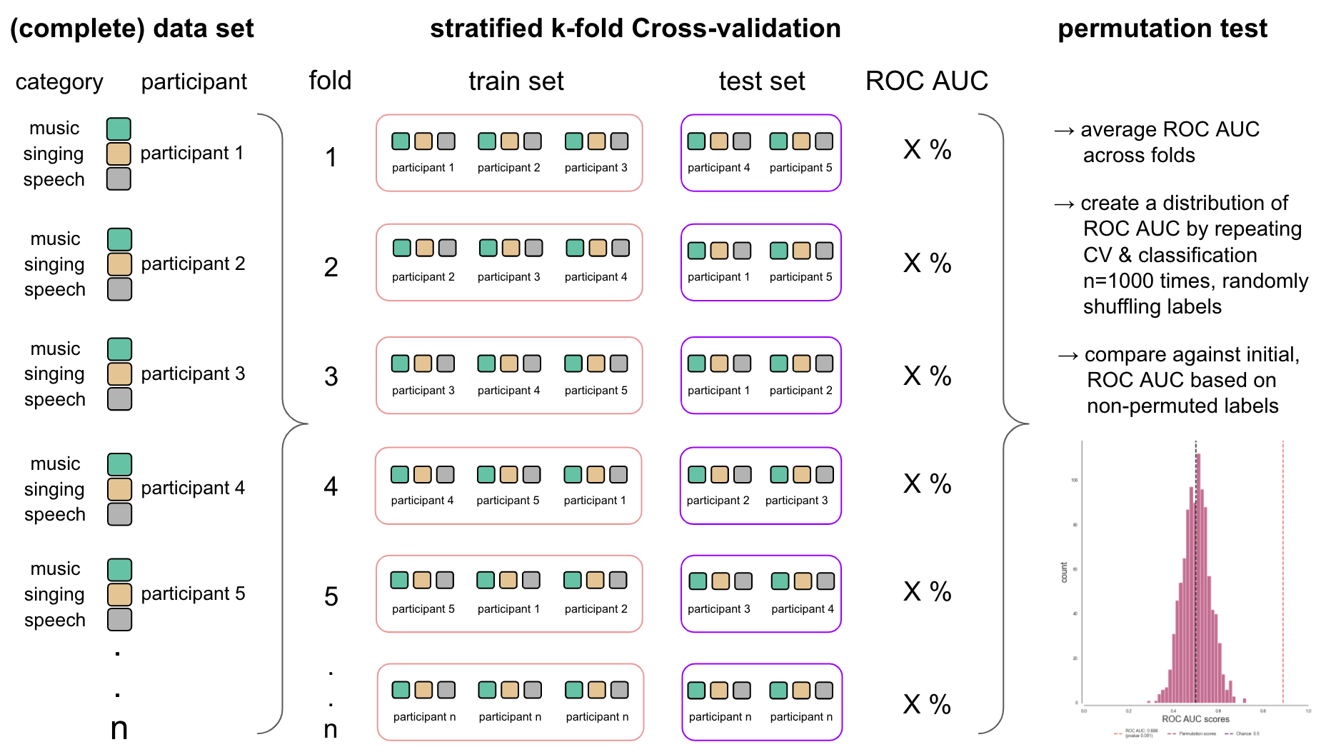
As you can see, there are a lot of steps required to define and set up our planned analyses. As we don’t want to iterate all these for each classification task, we’ll define some handy functions that combine respective parts in the next step.
defining analysis parameters - connecting the dots
Now that we have feature scaling, classifier, CV and permutation test in place, we can bring them together in one function that we can apply per classification task. This can be done using scikit-learn’s permutation_test_score function. It works like this (please note that this is a literate programming example):
permutation_test_score(estimator, features,
targets, scoring=scoring metric,
cv, n_permutations,
n_jobs, groups,
verbose=1)
Applied to our settings, the estimator will be our pipeline, features our con_images_data, targets our conditions, cv our CV, groups our participant labels and n_permutations=1000. So far, we’re missing the scoring metric. Within this project we decided to use Compute Area Under the Receiver Operating Characteristic Curve or ROC AUC for short. Given that we want to perform different binary and one multiclass classification task, we will include some small steps to restrict our dataset to the to be tested conditions. Our complete function thus looked like this:
def run_ROI_decoding(conditions_cl_task, roi=None, output_path=None):
'''
A small function to ease up the planned decoding tasks.
Providing the conditions to be tested and the ROI they should
be tested in, this function performs the decoding analysis and
the permutation test, as well as saves the outputs to disk.
Parameters
----------
conditions_cl_task : list
List of conditions to be tested
roi : path
Path to ROI conditions should be tested in
output_path : path
Path where results should be stored
'''
# generate condition mask to restrict the analysis to list of indicated conditions
condition_mask = conditions.isin(conditions_cl_task)
# set classification task name
if len(conditions_cl_task)==2:
task = '%sVS%s' %(conditions_cl_task[0],conditions_cl_task[1])
pipeline = make_pipeline(StandardScaler(), SVC(kernel='linear'))
scoring='roc_auc'
else:
task = 'multiclass'
pipeline = make_pipeline(StandardScaler(), SVC(kernel='linear', probability=True))
scoring='roc_auc_ovr'
# set output path
if output_path is None:
out_path = results_path
else:
out_path = output_path
if roi:
roi_masker = NiftiMasker(mask_img=roi, memory="nilearn_cache", memory_level=1)
con_images_data = roi_masker.fit_transform(con_images)
else:
roi_masker = NiftiMasker(mask_img=ac_mask, memory="nilearn_cache", memory_level=1)
con_images_data = roi_masker.fit_transform(con_images)
# restrict features, labels and participants to condition mask
con_image_data_task = con_images_data[condition_mask]
conditions_task = conditions[condition_mask]
participant_labels_task = participants[condition_mask]
# Confirm that we now have the conditions we indicated
print("analyzing the following conditions:", conditions_task.unique())
# run the analysis
score, permutation_scores, pvalue = permutation_test_score(pipeline, con_image_data_task,
pd.get_dummies(conditions_task)[conditions_cl_task[0]],
scoring=scoring,
cv=cv, n_permutations=1000,
n_jobs=3, groups=participant_labels_task,
verbose=1)
# Print the results
print("ROC AUC: %.4f / Chance level: %.2f / p value: %.4f" %
(score, 1. / len(conditions_task.unique()), pvalue))
# save results to disk
print('saving results to:', out_path)
permutation_results = {'task': task,
'accuracy (ROC AUC)': score,
'permutation_scores': permutation_scores.tolist(),
'p_value': pvalue}
if roi:
roi_str = roi[roi.rfind('c-')+2:roi.rfind('_mask')]
json.dump(permutation_results, open(opj(out_path, 'results/ROI',
"decoding_%s_space-MNI152NLin2009cAsym_desc-permutationscores_mask-%s.json" %(task, roi_str)),
'w' ))
else:
json.dump(permutation_results, open(opj(out_path,
"decoding_%s_space-MNI152NLin2009cAsym_desc-permutationscores_mask-AC.json" %task),
'w' ))
return permutation_results
It might look like a lot now, but it’s definitely better to set a comprehensive function once, than rerunning this steps for each classification task. Speaking of which: As we are also interested in how our classifiers perform, we will create a visualization function that plots the receiver operating characteristic curve across CV folds and the distribution of the permutation test scores in relation to the initial score. Again, it’s quite a long function, but the information is valuable.
def plot_classifier_performance(conditions_cl_task, permutation_results, interactive=False):
'''
A small function to visualize the decoding analysis
results. Two graphics will be generated: the ROC AUC
across folds and the permutation test scores.
Parameters
----------
conditions : list
List of conditions to be tested
permutation_results : dict
Outcomes of the run_ROI_decoding function
interactive : string
Inditicate if graphic should be static
or interactive.
'''
# generate condition mask to restrict the analysis to list of indicated conditions
condition_mask = conditions.isin(conditions_cl_task)
# set classification task name
if len(conditions_cl_task)==2:
task = '%sVS%s' %(conditions_cl_task[0],conditions_cl_task[1])
svc = SVC(kernel='linear')
else:
task = 'multiclass'
svc = OneVsRestClassifier(SVC(kernel='linear', probability=True,
decision_function_shape='ovo', random_state=42))
# restrict features, labels and participants to condition mask
con_image_data_task = con_images_data[condition_mask]
conditions_task = conditions[condition_mask]
participant_labels_task = participants[condition_mask]
# Confirm that we now have the conditions we indicated
print("plotting classifier performance for the following task:", conditions_task.unique())
tprs = []
aucs = []
mean_fpr = np.linspace(0, 1, 100)
con_data_task_scaled = StandardScaler().fit_transform(con_image_data_task, conditions_task)
cv = GroupShuffleSplit(n_splits=10, train_size=.8, random_state=42)
if interactive is True:
print("Currently not supported")
else:
sns.set_context('paper')
sns.set_style('white')
plt.rcParams["font.family"] = "Arial"
fig, axes = plt.subplots(1,2, figsize = (20, 10), sharex=True)
cpal = sns.color_palette('flare_r', 10)
for i, (train, test) in enumerate(cv.split(con_data_task_scaled, conditions_task, groups=participant_labels_task)):
svc.fit(con_data_task_scaled[train], conditions_task.to_numpy()[train])
viz = plot_roc_curve(svc, con_data_task_scaled[test], conditions_task.to_numpy()[test],
name='ROC fold {}'.format(i),
alpha=0.7, lw=1, color=cpal[i], ax=axes[0])
interp_tpr = np.interp(mean_fpr, viz.fpr, viz.tpr)
interp_tpr[0] = 0.0
tprs.append(interp_tpr)
aucs.append(viz.roc_auc)
axes[0].plot([0, 1], [0, 1], linestyle='--', lw=2, color='black',
label='Chance', alpha=.8)
mean_tpr = np.mean(tprs, axis=0)
mean_tpr[-1] = 1.0
mean_auc = auc(mean_fpr, mean_tpr)
std_auc = np.std(aucs)
axes[0].plot(mean_fpr, mean_tpr, color='black',
label=r'Mean ROC AUC = %0.2f $\pm$ %0.2f)' % (mean_auc, std_auc),
lw=2, alpha=.8)
std_tpr = np.std(tprs, axis=0)
tprs_upper = np.minimum(mean_tpr + std_tpr, 1)
tprs_lower = np.maximum(mean_tpr - std_tpr, 0)
axes[0].fill_between(mean_fpr, tprs_lower, tprs_upper, color='grey', alpha=.2,
label=r'$\pm$ 1 std. dev.')
axes[0].set(xlim=[-0.05, 1.05], ylim=[-0.05, 1.05])
axes[0].legend(loc="lower right", bbox_to_anchor=(1.05,0), frameon=False)
axes[0].set_xlabel('False Positive Rate', fontsize=18)
axes[0].set_ylabel('True Positive Rate', fontsize=18)
plt.text(-1.4,123, "Receiver operating characteristic for classification task %s" %task, fontsize=16)
# View histogram of permutation scores
sns.histplot(permutation_results['permutation_scores'], color=sns.color_palette("flare_r")[2], ax=axes[1])
sns.despine(offset=5)
ylim = plt.ylim()
xlim = ([0,1])
plt.plot(2 * [permutation_results['accuracy (ROC AUC)']], ylim, color=sns.color_palette("flare_r")[4],
linewidth=2, linestyle='dashed')
plt.plot(2 * [1. / len(conditions_task.unique())], ylim, color='k', linewidth=2, linestyle='dashed')
plt.ylim(ylim)
plt.xlim(xlim)
plt.xlabel('ROC AUC scores', fontsize=18)
plt.ylabel('count', fontsize=18)
custom_lines = [Line2D([0], [0], color=sns.color_palette("flare_r")[4], lw=2, linestyle='dashed'),
Line2D([0], [0], color=sns.color_palette("flare_r")[2], lw=2, linestyle='dashed'),
Line2D([0], [0], color=sns.color_palette("flare_r")[0], lw=2, linestyle='dashed')]
plt.legend(custom_lines, ['ROC AUC: %s \n(pvalue %s)'
%(round(permutation_results['accuracy (ROC AUC)'], 3),
round(permutation_results['p_value'],4)),
'Permutation scores',
'Chance: 0.5'],
loc="lower right", bbox_to_anchor=(0.8,-0.15), ncol=3, frameon=False)
plt.text(-0.001,123, "Permutation test score for classification task %s" %task, fontsize=16)
plt.subplots_adjust(wspace=0.4)
fig.suptitle('Classifier performance and permutation test for classification task %s within the auditory cortex ROI' %task, size=20)
plt.show()
Ok, time to go to work and start our analyses, beginning with searchlights.
Searchlight analyses
The first set of the conducted MVPA entails multiple searchlight analysis. Our goal here was to identify regions of the auditory cortex that carry information with regard to a certain classification task. Searchlight analysis achieve this goal via performing a given classification task at multiple locations, here within the auditory cortex. To this end, a small sphere travels through the volume of interest and at each point extracts the corresponding voxel pattern, performs the classification task and assigns the center voxel of the sphere the obtained scoring metric. Termed infomration based mapping we therefore get searchlight maps that exhibit the scoring performance of regions/voxels. We can implement this analysis using nilearn’s Searchlight class. It basically takes the same input arguments as the permutation_test_score function we defined above, but also needs a mask_img and a process_mask_img that define the parts of the brain we want to restrict our searchlight to. No surprise: for us that’s the auditory cortex mask. Another important parameter to set is the radius, that is the size of our sphere. We’re going to use a radius of 4 based on prior research that suggested this value as a reasonable default [REF]. As mentioned in the permutation test secion: assessing the significance of searchlight outcomes can be more tricky than e.g. ROI decoding. While previous research work employed parametric tests (for example against chance level), work on simulated and real data [REF] provided evidence that this option is not favourable. Instead, permutation tests should be used for these analyses as well. One promising approach was introduced by [REF] and constitutes to generate a set of searchlight maps based on permuted data and then submit those to a group level analysis. As outlined in the previous section, we can unfortunately not conduct a sufficient within participant CV as we only have two runs and thus need to CV across participants. As this means we can also not implement the approach of [REF], we decided to go with two complementary alternatives. First, we employed a mixture of the described ROI decoding approach and classic searchlights. In more detail, we shuffled the labels and run the searchlight analysis on this permuted data. Through repeating this step e.g. 1000 times, we create a distribution of scores for each voxel (i.e. searchlight center) and then can count how often the permuted score is higher than the original score following the same hypothesis of label-feature dependency as explained above. With that we get a map that contains p-values for each voxel. However, as you might have heard, there’s this thing called multiple-comparison correction that is required to correct inflated p-values in case of many tests. Even though we restricted our analyses to the auditory cortex, we still have a lot of tests, i.e. ~ 9.5k voxels as we saw earlier. Thus it might be a good idea to account for it and apply correction for multiple comparisons. To this end, we will transform the p-value searchlight map to a z-value searchlight map and subsequently apply a correction method, more precisely [False Discovery Rate](). With that we will get a map that shows us regions that can perform the classification tasks significantly better than chance. The second alternative is based on [REF]. For each searchlight analyses we run the same classification task in an ROI decoding approach where we treated the auditory cortex mask as one ROI in order to evaluate if the patterns we use for the searchlight analyses contain respective information. Identical to the ROI decoding we run 1000 permutations for each classification task. Comparable to the ROI decoding and results visualization, we will set up a small function that performs the necessary steps for us. This includes defining the searchlight, fitting the searchlight to our images, performing permutation tests and creating new images entailing the results. As outlined above, we used the same CV and pipeline throughout all analyses, thus we also set them here accordingly. Please note, that the second permutation test (i.e. treating the auditory cortex as one ROI) will be carried out using the ROI_decoding function.
def run_searchlight_analysis(conditions_cl_task, output_path=None, permutation_test=False, n_permutations=None):
'''
A small function to ease up the planned searchlight analyses.
Providing the conditions to be tested, this function performs
the searchlight analysis, as well as saves the outputs to disk
and visualizes the results.
Parameters
----------
conditions_cl_task : list
List of conditions to be tested
output_path : path
Path where results should be stored
permutation_test : bool
If True permutation tests will be performed.
Default: False.
n_permutations: int
If permutation_test=True, the number of permutations
needs to be set. E.g. n_permutations=100 .
'''
# set classification task name and pipeline settings
# for binary or multiclass task
if len(conditions_cl_task)==2:
task = '%sVS%s' %(conditions_cl_task[0],conditions_cl_task[1])
pipeline = make_pipeline(StandardScaler(), SVC(kernel='linear'))
scoring='roc_auc'
else:
task = 'multiclass'
pipeline = make_pipeline(StandardScaler(), SVC(kernel='linear', probability=True))
scoring='roc_auc_ovr'
# set cross validation across participants
cv = GroupShuffleSplit(n_splits=10, train_size=.8, random_state=42)
# set output path
if output_path is None:
out_path = results_path
else:
out_path = output_path
# generate condition mask to restrict the analysis to list of indicated conditions
condition_mask = conditions.isin(conditions_cl_task)
# restrict images to those needed for the classification task
con_images_task = index_img(con_images, condition_mask)
# restrict conditions to those needed for the classification task
conditions_task = conditions[condition_mask]
# restrict participants to those needed for the classification task
participant_labels_task = participants[condition_mask]
# define the searchlight
searchlight_unfit = SearchLight(ac_mask,
process_mask_img=ac_mask,
radius=4, n_jobs=2,
verbose=1, cv=cv,
estimator=pipeline, scoring=scoring)
searchlight_orig = clone(searchlight_unfit)
# print information to check if searchlight runs correctly specified
print("performing searchlight for classification task:", task)
# apply the searchlight
searchlight_orig.fit(con_images_task, conditions_task, groups=participant_labels_task)
# generate image containing results and save to disk
searchlight_img_orig = new_img_like(ac_mask, searchlight_orig.scores_)
searchlight_img_orig.to_filename(opj(out_path, 'searchlightmap_%s_space-MNI152NLin2009cAsym.nii.gz' %task))
np.save(opj(out_path, 'searchlightmap_%s_space-MNI152NLin2009cAsym_desc-origscores.npy' %task), searchlight_orig.scores_)
# print the output path
print("searchlight map will be saved to:", out_path)
# if permutation tests shoul be run, do it
if permutation_test:
# check if number of permutations was set, if not stop
if not n_permutations:
print("You specified that you want to run a permutation test to assess significance. However, you did not"\
"indicate the number of permutations that should be run. Please do so via the n_permutations argument.")
# load searchlight mask for storing permutation scores
ac_mask_data = get_data(ac_mask)
ac_mask_voxels = ac_mask_data[ac_mask_data==1]
ac_masker = NiftiMasker(mask_img=ac_mask, memory="nilearn_cache", memory_level=1)
_ = ac_masker.fit_transform(con_images_task)
# initiate permutation searchlight score array
permutation_searchlight_scores = np.empty((n_permutations, ac_mask_voxels.shape[0]))
# loop over number of permutations
for i in range(n_permutations):
print('permutation: %s/%s' %(str(i), str(n_permutations)))
# reset searchlight based on original one
searchlight_perm = clone(searchlight_unfit)
# initiate random shuffle for each permutation to make it reproducible
rng = np.random.default_rng(i)
# set empty list for shuffled conditions
list_conditions_shuffled = []
# for each participant randomly shuffle lables
for part in range(23):
list_conditions_shuffled.extend(rng.permutation(conditions_cl_task))
# run searchlight on permuted data
searchlight_perm.fit(con_images_task, list_conditions_shuffled, groups=participant_labels_task)
# save permutation scores of respective permutation in dictionary
permutation_searchlight_scores[i] = searchlight_perm.scores_[ac_mask_data==1]
# save permutation results
np.save(opj(results_path, 'searchlightmap_%s_space-MNI152NLin2009cAsym_desc-permutations.npy'), permutation_searchlight_scores)
# count how often permuted scores were higher than original score per voxel
# do the same for the max value within each permutation
count_orig_perm = np.zeros(shape=searchlight_orig.scores_[ac_mask_data==1].shape[0])
count_orig_perm_max = np.zeros(shape=searchlight_orig.scores_[ac_mask_data==1].shape[0])
for i in range(len(permutation_searchlight_scores)):
count_orig_perm[permutation_searchlight_scores[i] >= searchlight_orig.scores_[ac_mask_data==1]] += 1
count_orig_perm_max[np.max(permutation_searchlight_scores[i]) >= searchlight_orig.scores_[ac_mask_data==1]] += 1
# save max value array and image
count_orig_perm_max_p = (count_orig_perm_max + 1) / (n_permutations + 1)
np.save(opj(out_path, 'searchlightmap_%s_space-MNI152NLin2009cAsym_desc-perm-%s-maxscores.npy' %(task, n_permutations)), count_orig_perm_max)
searchlight_img_p_max = ac_masker.inverse_transform(count_orig_perm_max_p)
searchlight_img_p_max.to_filename(opj(out_path, 'searchlightmap_%s_space-MNI152NLin2009cAsym_desc-perm-%s-pmax.nii.gz' %(task, n_permutations)))
# compute uncorrecpted p values for each voxel via dividing count by number of permutations, then save array and image
count_orig_perm_p_uncor = (count_orig_perm + 1) / (n_permutations + 1)
np.save(opj(out_path, 'searchlightmap_%s_space-MNI152NLin2009cAsym_desc-perm-%s-uncorp.npy' %(task, n_permutations)), count_orig_perm_p_uncor)
searchlight_img_p_uncor = ac_masker.inverse_transform(count_orig_perm_p_uncor)
searchlight_img_p_uncor.to_filename(opj(out_path, 'searchlightmap_%s_space-MNI152NLin2009cAsym_desc-perm-%s-uncorp.nii.gz' %(task, n_permutations)))
# compute z values for each voxel, then save array and image
count_orig_perm_z = st.norm.isf(count_orig_perm_p_uncor)
np.save(opj(out_path, 'searchlightmap_%s_space-MNI152NLin2009cAsym_desc-perm-%s-Zscores.npy' %(task, n_permutations)), count_orig_perm_z)
searchlight_img_z = ac_masker.inverse_transform(count_orig_perm_z)
searchlight_img_z.to_filename(opj(out_path, 'searchlightmap_%s_space-MNI152NLin2009cAsym_desc-perm-%s-zmap.nii.gz' %(task, n_permutations)))
# compute mean values for each voxel across permutations, then save array and image
mean_permutation_scores = np.mean(permutation_searchlight_scores, axis=0)
np.save(opj(out_path, 'searchlightmap_%s_space-MNI152NLin2009cAsym_desc-perm-%s-meanscores.npy' %(task, n_permutations)), mean_permutation_scores)
searchlight_img_mean = ac_masker.inverse_transform(mean_permutation_scores)
searchlight_img_mean.to_filename(opj(out_path, 'searchlightmap_%s_space-MNI152NLin2009cAsym_desc-perm-%s-meanmap.nii.gz' %(task, n_permutations)))
# compute std values for each voxel across permutations, then save array and image
std_permutation_scores = np.std(permutation_searchlight_scores, axis=0)
np.save(opj(out_path, 'searchlightmap_%s_space-MNI152NLin2009cAsym_desc-perm-%s-stdscores.npy' %(task, n_permutations)), std_permutation_scores)
searchlight_img_std = ac_masker.inverse_transform(std_permutation_scores)
searchlight_img_std.to_filename(opj(out_path, 'searchlightmap_%s_space-MNI152NLin2009cAsym_desc-perm-%s-stdmap.nii.gz' %(task, n_permutations)))
return (searchlight_img_orig, searchlight_orig.scores_, permutation_searchlight_scores, count_orig_perm_z, count_orig_perm_max) if permutation_test else (searchlight_img_orig, searchlight_orig.scores_)
That’s quite a function, eh? Luckily, we can just call it from now on. What we are missing for our searchlight analyses is a function that provides informative visualizations of results. As before, nilearn has our back and we can easily get static or interactive plots. In either case, we will plot the original searchlight map and overlay the thresholded permutation test based z-value searchlight map to indicate regions with significant results. Thus, we will also include some code that applies the multiple comparison correction we talked about, namely FDR, to the z-value searchlight maps from the permutation test and saves the thresholded maps as binary masks.
def plot_searchlight_results(searchlight_map, permutation_map=None, alpha=0.05, interactive=False, surface=False):
'''
A small function to ease up visualization of the searchlight results.
Providing the original searchlight mask and the z-value searchlight map
obtained through permutation tests, this function applies multiple comparison
corerction to the z-value map and creates a binary mask from this thresholded
map, which will then be plotted on top of the original searchlight map.
Parameters
----------
searchlight_map : path
Original searchlight map
permutation_map : path
Z-value searchlight map obtained through permutation test
alpha : float
Alpha level for multiple comparion correction.
Default: 0.05.
interactive: bool
If interactive=True, an interactive graphic will be generated.
Default=False
'''
task = searchlight_map[searchlight_map.rfind('map_')+4:searchlight_map.rfind('_space')]
searchlight_map=nb.load(searchlight_map)
if permutation_map:
permutation_map=nb.load(permutation_map)
# get threshold given z-values and alpha, borrowed from nilearn
if alpha < 0 or alpha > 1:
raise ValueError(
'alpha should be between 0 and 1. {} was provided'.format(alpha))
z_vals_ = - np.sort(- get_data(permutation_map))
p_vals = st.norm.sf(z_vals_)
n_samples = len(p_vals)
pos = p_vals < alpha * np.linspace(
.5 / n_samples, 1 - .5 / n_samples, n_samples)
if pos.any():
threshold = (z_vals_[pos][-1] - 1.e-12)
else:
threshold = np.infty
threshold_z_values = threshold_img(permutation_map, threshold=threshold)
threshold_z_values_mask = math_img('img > 0', img=threshold_z_values)
threshold_z_values_mask.header.set_data_dtype(np.uint8)
threshold_z_values_mask.to_filename(opj(results_path, 'results/searchlight', 'searchlightmap_%s_space-MNI152NLin2009cAsym_desc-perm-1000-zmap_mask.nii.gz' %task))
threshold_searchlight_map = threshold_img(searchlight_map, threshold=0.5)
if interactive is True and surface is False:
fig = view_img(threshold_searchlight_map, cmap='flare_r', title = 'Searchlight analyses - %s searchlight map' %task)
return fig
elif interactive is True and surface is True:
fig = view_img_on_surf(threshold_searchlight_map, threshold=0.0001, cmap='flare_r', colorbar=True,
title="%s searchlight map" %task, symmetric_cmap=False)
return fig
else:
fig=plt.figure(num=None, figsize=(12, 6))
searchlight_plot = plot_img(threshold_searchlight_map, cmap='flare_r', cut_coords=[-60, -34, 7], threshold=0.5,
bg_img=load_mni152_template(), draw_cross=False, colorbar=False, figure=fig)
searchlight_plot.add_contours(threshold_z_values_mask, alpha=0.7, colors='black', linewidths=0.5)
plt.text(-300, 90, 'Searchlight analyses - %s searchlight map' %task, fontsize=20)
Looks about right. With all functions we need define, we ready to actually run the searchlight analysis. Very important: Given that this resource aims to document the analyses as detailed as possible in an interactive manner, we won’t run the permutation tests, but only the original searchlight analyses here. This is based on two reasons: 1) we decided to go with 1k permutations for a given classification task and each took ~11 hours running on a powerful HPC with 20 cores; 2) despite the very long duration, we also can’t set up a comparable computationally infrastructure folks can use interactively, but are bound to resource allocations available via binder. Please don’t get this wrong, binder is fantastic and we all should be so glad to have this amazing resource that additionally nicely integrates with jupyter hub. At the time this resource was created, there were just limits on what could be run where. Assuming that more folks support binder or create local hubs in the future, the types of analyses that can be run will definitely increase, including those that are computationally very heavy. Thus, at this point in time, we provide the results of searchlight analyses with permutation tests through the project’s OSF repository which you can download as shown before for the contrast images via the osf client. Within that, you will also find the analysis scripts we run on our HPC if you really want to re-run these analyses yourself. In contrast, the second option of significance testing, i.e. using the auditory cortex mask within the ROI decoding approach should be working. Thus, if you have time and feel like it, you can run this part interactively here. The results will however also be downloaded from OSF as well.
osf -p <projectid> fetch remote/path.txt local/file.txt
Ok ok ok, nuff said, let’s finally start with the actual analyses, beginning with the multiclass classification task.
Searchlight analyses - Multiclass
For the first classification task we are going to evaluate which voxels/regions carry information regarding the distinction of all categories. Given our nice functions, we know only need a few lines of code to run the analysis. Our input for the first step, the searchlight analyses itself, will be ['music', 'singing', 'speech'].
searchlight_multiclass = run_searchlight_analysis(['music', 'singing', 'voice'], output_path=None)
performing searchlight for classification task: multiclass
[Parallel(n_jobs=2)]: Using backend LokyBackend with 2 concurrent workers.
[Parallel(n_jobs=2)]: Done 2 out of 2 | elapsed: 14.9min remaining: 0.0s
[Parallel(n_jobs=2)]: Done 2 out of 2 | elapsed: 14.9min finished
searchlight map will be saved to: /data/mvs/derivatives/MVPA/
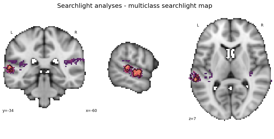
Fantastic, now we can use our visualization function to check out the results. At first, on the inflated surfaceto get a basic explorative overview.
plot_searchlight_results(opj(results_path, 'results/searchlight/searchlightmap_multiclass_space-MNI152NLin2009cAsym.nii.gz'), interactive=True, surface=True)
And now a bit more detailed with the permutation results overlaid on the searchlight map:
plot_searchlight_results(opj(results_path, 'results/searchlight/searchlightmap_multiclass_space-MNI152NLin2009cAsym.nii.gz'),
opj(results_path, 'results/searchlight/searchlightmap_multiclass_space-MNI152NLin2009cAsym_desc-perm-1000-zmap.nii.gz'),
alpha=0.05)
The next step is to compute the classification performance and its significance for the multiclass classification task using the auditory cortex mask. This is rather straightforward using our corresponding function:
deocding_permutation_results_multiclass = run_ROI_decoding(['music', 'singing', 'voice'])
analyzing the following conditions: ['music' 'singing' 'voice']
[Parallel(n_jobs=3)]: Using backend LokyBackend with 3 concurrent workers.
[Parallel(n_jobs=3)]: Done 44 tasks | elapsed: 30.8s
[Parallel(n_jobs=3)]: Done 194 tasks | elapsed: 2.2min
[Parallel(n_jobs=3)]: Done 444 tasks | elapsed: 4.8min
[Parallel(n_jobs=3)]: Done 794 tasks | elapsed: 8.4min
ROC AUC: 0.8500 / Chance level: 0.5 / p value: 0.0010
saving results to: /data/mvs/derivatives/MVPA/
[Parallel(n_jobs=3)]: Done 1000 out of 1000 | elapsed: 10.5min finished
Now, we can use our visualization function to inspect the results.
plot_classifier_performance(['music', 'singing', 'voice'], deocding_permutation_results_multiclass)
That looks about right, cool. Let’s continue with the other classification tasks.
Searchlight analyses - music vs. voice
Next up is the music vs. voice classification task
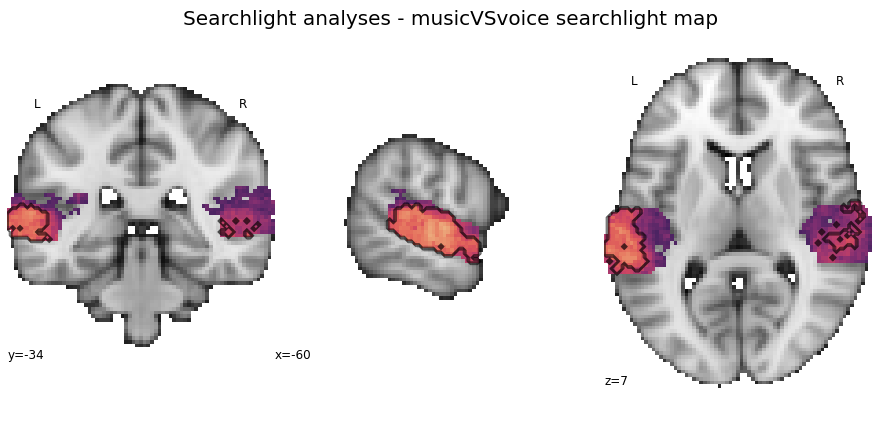
searchlight_musicVSvoice = run_searchlight_analysis(['music', 'voice'], output_path=opj(results_path, 'results'))
performing searchlight for classification task: musicVSvoice
[Parallel(n_jobs=3)]: Using backend LokyBackend with 3 concurrent workers.
[Parallel(n_jobs=3)]: Done 3 out of 3 | elapsed: 3.2min finished
searchlight map will be saved to: /data/mvs/derivatives/MVPA/results
How do the results look like? We start with the interactive surface plot again:
plot_searchlight_results(opj(results_path, 'results/searchlight/searchlightmap_musicVSvoice_space-MNI152NLin2009cAsym.nii.gz'), interactive=True, surface=True)
And here is the detailed version including permutation test results:
plot_searchlight_results(opj(results_path, 'results/searchlight/searchlightmap_musicVSvoice_space-MNI152NLin2009cAsym.nii.gz'),
opj(results_path, 'results/searchlight/searchlightmap_musicVSvoice_space-MNI152NLin2009cAsym_desc-perm-1000-zmap.nii.gz'),
alpha=0.05)
The ROI decoding approach is up next.
deocding_permutation_results_musicVSspeech = run_ROI_decoding(['music', 'voice'], output_path=opj(results_path, 'results'))
analyzing the following conditions: ['music' 'voice']
[Parallel(n_jobs=3)]: Using backend LokyBackend with 3 concurrent workers.
[Parallel(n_jobs=3)]: Done 44 tasks | elapsed: 5.9s
[Parallel(n_jobs=3)]: Done 194 tasks | elapsed: 23.7s
[Parallel(n_jobs=3)]: Done 444 tasks | elapsed: 52.2s
[Parallel(n_jobs=3)]: Done 794 tasks | elapsed: 1.8min
ROC AUC: 0.8880 / Chance level: 0.50 / p value: 0.0010
saving results to: /data/mvs/derivatives/MVPA/results
[Parallel(n_jobs=3)]: Done 1000 out of 1000 | elapsed: 2.2min finished
And here’s how our results look like:
plot_classifier_performance(['music', 'voice'], deocding_permutation_results_musicVSspeech)
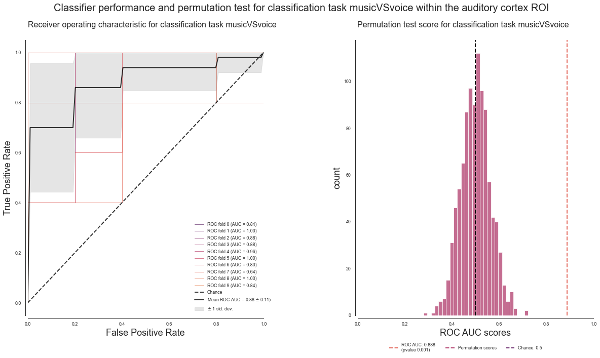
Let’s keep it short: LGTM.
Searchlight analyses - music vs. singing
We are already at the music vs. singing classification task.
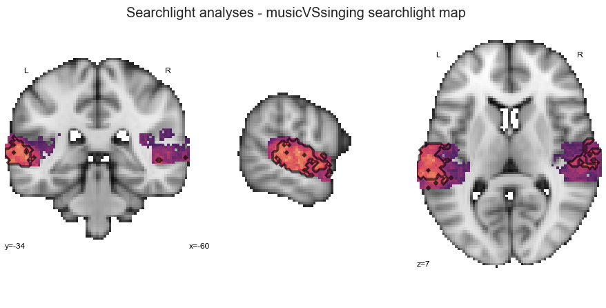
searchlight_musicVSsinging = run_searchlight_analysis(['music', 'singing'], output_path=opj(results_path, 'results'))
performing searchlight for classification task: musicVSsinging
[Parallel(n_jobs=2)]: Using backend LokyBackend with 2 concurrent workers.
[Parallel(n_jobs=2)]: Done 2 out of 2 | elapsed: 3.8min remaining: 0.0s
[Parallel(n_jobs=2)]: Done 2 out of 2 | elapsed: 3.8min finished
searchlight map will be saved to: /data/mvs/derivatives/MVPA/results
Show me the outcomes please, interactive surface plot first, detailed plot wit permutation test results second:
plot_searchlight_results(opj(results_path, 'results/searchlight/searchlightmap_musicVSsinging_space-MNI152NLin2009cAsym.nii.gz'), interactive=True, surface=True)
plot_searchlight_results(opj(results_path, 'results/searchlight/searchlightmap_musicVSsinging_space-MNI152NLin2009cAsym.nii.gz'),
opj(results_path, 'results/searchlight/searchlightmap_musicVSsinging_space-MNI152NLin2009cAsym_desc-perm-1000-zmap.nii.gz'),
alpha=0.05)
Subsequently, we will run the ROI decoding approach:
deocding_permutation_results_musicVSsinging = run_ROI_decoding(['music', 'singing'], output_path=opj(results_path, 'results'))
analyzing the following conditions: ['music' 'singing']
[Parallel(n_jobs=3)]: Using backend LokyBackend with 3 concurrent workers.
[Parallel(n_jobs=3)]: Done 44 tasks | elapsed: 5.8s
[Parallel(n_jobs=3)]: Done 194 tasks | elapsed: 23.1s
[Parallel(n_jobs=3)]: Done 444 tasks | elapsed: 52.2s
[Parallel(n_jobs=3)]: Done 794 tasks | elapsed: 1.8min
ROC AUC: 0.8040 / Chance level: 0.50 / p value: 0.0010
saving results to: /data/mvs/derivatives/MVPA/results
[Parallel(n_jobs=3)]: Done 1000 out of 1000 | elapsed: 2.2min finished
And check its outcomes:
plot_classifier_performance(['music', 'singing'], deocding_permutation_results_musicVSsinging)
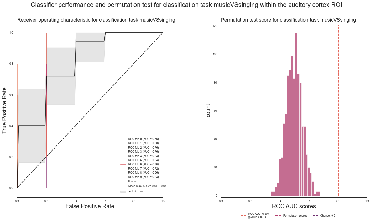
Nice, comparable to the previous classification tasks.
Searchlight analyses voice vs. singing
And the last classification task within the searchlight analyses: voice vs. singing.
searchlight_voiceVSsinging = run_searchlight_analysis(['voice', 'singing'], output_path=opj(results_path, 'results'))
performing searchlight for classification task: voiceVSsinging
[Parallel(n_jobs=2)]: Using backend LokyBackend with 2 concurrent workers.
[Parallel(n_jobs=2)]: Done 2 out of 2 | elapsed: 3.7min remaining: 0.0s
[Parallel(n_jobs=2)]: Done 2 out of 2 | elapsed: 3.7min finished
searchlight map will be saved to: /data/mvs/derivatives/MVPA/results
How are the results looking? As done before, we are going to start with the interactive surface plot:
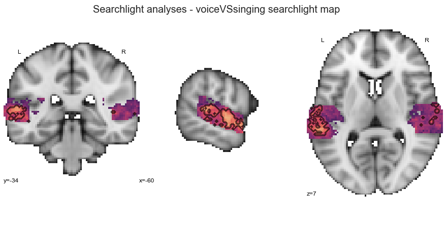
plot_searchlight_results(opj(results_path, 'results/searchlight/searchlightmap_voiceVSsinging_space-MNI152NLin2009cAsym.nii.gz'), interactive=True, surface=True)
And here is the detailed version with permutation test results:
plot_searchlight_results(opj(results_path, 'results/searchlight/searchlightmap_voiceVSsinging_space-MNI152NLin2009cAsym.nii.gz'),
opj(results_path, 'results/searchlight/searchlightmap_voiceVSsinging_space-MNI152NLin2009cAsym_desc-perm-1000-zmap.nii.gz'),
alpha=0.05)
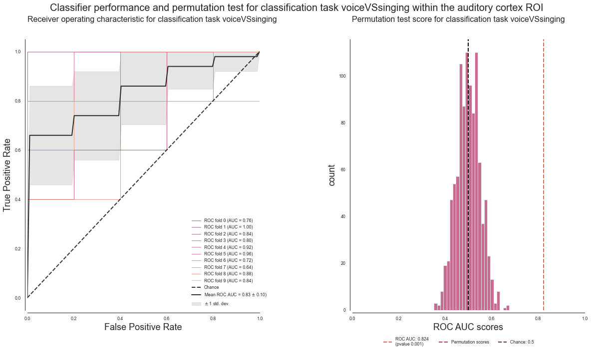
What about the ROI decoding approach?
deocding_permutation_results_voiceVSsinging = run_ROI_decoding(['voice', 'singing'], output_path=opj(results_path, 'results'))
analyzing the following conditions: ['singing' 'voice']
[Parallel(n_jobs=3)]: Using backend LokyBackend with 3 concurrent workers.
[Parallel(n_jobs=3)]: Done 44 tasks | elapsed: 4.7s
[Parallel(n_jobs=3)]: Done 194 tasks | elapsed: 21.1s
[Parallel(n_jobs=3)]: Done 444 tasks | elapsed: 49.4s
[Parallel(n_jobs=3)]: Done 794 tasks | elapsed: 1.6min
ROC AUC: 0.8240 / Chance level: 0.50 / p value: 0.0010
saving results to: /data/mvs/derivatives/MVPA/results
[Parallel(n_jobs=3)]: Done 1000 out of 1000 | elapsed: 2.0min finished
The results for this classification task look as follows:
plot_classifier_performance(['voice', 'singing'], deocding_permutation_results_voiceVSsinging)
Searchlight analyses - comparison of tasks
Now that we run all classification tasks, let’s visualize the performance of the ROI decoding approach within the auditory mask across all tasks to get a sense how they compare to one another. To do so, we start by loading the above defined and saved classification task specific json files. For each classification task we will load the corresponding json file and set the respective values, including the permutation scores, the ROC AUC and p value.
Multiclass classification task
with open(opj(results_path, 'results/searchlight',
"decoding_multiclass_space-MNI152NLin2009cAsym_desc-permutationscores.json"),
'r' ) as multiclass_data:
permutation_data_multiclass = json.load(multiclass_data)
permutation_scores_multiclass = permutation_data_multiclass['permutation_scores']
accuracy_multiclass = permutation_data_multiclass['accuracy (ROC AUC)']
p_value_multiclass = permutation_data_multiclass['p_value']
Music vs voice classification task
with open(opj(results_path, 'results/searchlight',
"decoding_musicVSvoice_space-MNI152NLin2009cAsym_desc-permutationscores.json"),
'r' ) as musicVSvoice_data:
permutation_data_musicVSvoice = json.load(musicVSvoice_data)
permutation_scores_musicVSvoice = permutation_data_musicVSvoice['permutation_scores']
accuracy_musicVSvoice = permutation_data_musicVSvoice['accuracy (ROC AUC)']
p_value_musicVSvoice = permutation_data_musicVSvoice['p_value']
Music vs singing classification task
with open(opj(results_path, 'results/searchlight',
"decoding_musicVSsinging_space-MNI152NLin2009cAsym_desc-permutationscores.json"),
'r' ) as musicVSsinging_data:
permutation_data_musicVSsinging = json.load(musicVSsinging_data)
permutation_scores_musicVSsinging = permutation_data_musicVSsinging['permutation_scores']
accuracy_musicVSsinging = permutation_data_musicVSsinging['accuracy (ROC AUC)']
p_value_musicVSsinging = permutation_data_musicVSsinging['p_value']
Voice vs singing classification task
with open(opj(results_path, 'results/searchlight',
"decoding_voiceVSsinging_space-MNI152NLin2009cAsym_desc-permutationscores.json"),
'r' ) as voiceVSsinging_data:
permutation_data_voiceVSsinging = json.load(voiceVSsinging_data)
permutation_scores_voiceVSsinging = permutation_data_voiceVSsinging['permutation_scores']
accuracy_voiceVSsinging = permutation_data_voiceVSsinging['accuracy (ROC AUC)']
p_value_voiceVSsinging = permutation_data_voiceVSsinging['p_value']
Now that we have everything back in memory, we pack them all together in one DataFrame to ease up the generation of the planned graphic:
permutation_scores_all = pd.DataFrame({'task': 1000 * ['multiclass']
+ 1000 * ['music vs voice']
+ 1000 * ['music vs singing']
+ 1000 * ['voice vs singing'],
'permutation score' : permutation_scores_multiclass
+ permutation_scores_musicVSvoice
+ permutation_scores_musicVSsinging
+ permutation_scores_voiceVSsinging})
Let’s make sure the DataFrame turned out as expected:
permutation_scores_all
| task | permutation score | |
|---|---|---|
| 0 | multiclass | 0.464 |
| 1 | multiclass | 0.498 |
| 2 | multiclass | 0.540 |
| 3 | multiclass | 0.554 |
| 4 | multiclass | 0.448 |
| 5 | multiclass | 0.378 |
| 6 | multiclass | 0.508 |
| 7 | multiclass | 0.450 |
| 8 | multiclass | 0.472 |
| 9 | multiclass | 0.534 |
| 10 | multiclass | 0.558 |
| 11 | multiclass | 0.558 |
| 12 | multiclass | 0.510 |
| 13 | multiclass | 0.558 |
| 14 | multiclass | 0.486 |
| 15 | multiclass | 0.442 |
| 16 | multiclass | 0.506 |
| 17 | multiclass | 0.492 |
| 18 | multiclass | 0.502 |
| 19 | multiclass | 0.460 |
| 20 | multiclass | 0.390 |
| 21 | multiclass | 0.590 |
| 22 | multiclass | 0.476 |
| 23 | multiclass | 0.546 |
| 24 | multiclass | 0.482 |
| 25 | multiclass | 0.450 |
| 26 | multiclass | 0.540 |
| 27 | multiclass | 0.458 |
| 28 | multiclass | 0.494 |
| 29 | multiclass | 0.536 |
| ... | ... | ... |
| 3970 | voice vs singing | 0.536 |
| 3971 | voice vs singing | 0.500 |
| 3972 | voice vs singing | 0.428 |
| 3973 | voice vs singing | 0.452 |
| 3974 | voice vs singing | 0.524 |
| 3975 | voice vs singing | 0.552 |
| 3976 | voice vs singing | 0.536 |
| 3977 | voice vs singing | 0.676 |
| 3978 | voice vs singing | 0.460 |
| 3979 | voice vs singing | 0.480 |
| 3980 | voice vs singing | 0.404 |
| 3981 | voice vs singing | 0.536 |
| 3982 | voice vs singing | 0.504 |
| 3983 | voice vs singing | 0.552 |
| 3984 | voice vs singing | 0.460 |
| 3985 | voice vs singing | 0.460 |
| 3986 | voice vs singing | 0.476 |
| 3987 | voice vs singing | 0.528 |
| 3988 | voice vs singing | 0.520 |
| 3989 | voice vs singing | 0.416 |
| 3990 | voice vs singing | 0.484 |
| 3991 | voice vs singing | 0.472 |
| 3992 | voice vs singing | 0.444 |
| 3993 | voice vs singing | 0.424 |
| 3994 | voice vs singing | 0.544 |
| 3995 | voice vs singing | 0.552 |
| 3996 | voice vs singing | 0.424 |
| 3997 | voice vs singing | 0.588 |
| 3998 | voice vs singing | 0.484 |
| 3999 | voice vs singing | 0.456 |
4000 rows × 2 columns
Cool, we have 4k rows and 2 columns: 1000 permutation scores for each of 4 classification tasks. That’s exactly what we want and thus we can continue.
As said before: graphics and their colormaps are very important. Hence, we will use an appropriate colormap (i.e. flare_r, the one we are using throughout the MVPA part of this project) and raincloud plots. to convey as much information as possible. In more detail, we will plot the ROC AUC score of each permutation via a scatter plot and on top of that median, std and outliers via boxplots. The cherry on the cake will be a histogram plotted above the scatter/box plot combination. As you will see this will resemble a cloud (the histogram) from which it is raining (the scatter plot), thus a raincloud plot. Isn’t data and its visualization beautiful? To add even more information we will include a dotted line indicating the chance level, as well as markers for each original ROC AUC score to show the distinction to permutation ROC AUC scores.
sns.set_context('paper')
sns.set_style('white')
plt.rcParams["font.family"] = "Arial"
dx="task"; dy="permutation score"; ort="h"; pal = "Set2"; sigma = .2
f, ax = plt.subplots(figsize=(15, 8))
ax=pt.RainCloud(x = dx, y = dy, data = permutation_scores_all, palette = 'flare_r', bw = sigma,
width_viol = .5, ax = ax, orient = ort)#, **font)
plt.xlabel('ROC AUC scores based on label permutations (n=1000)', fontsize=16)
plt.ylabel('classification task', fontsize=16)
plt.title('Permutation test scores across classification tasks within auditory cortex mask', fontsize=18)
plt.scatter(accuracy_multiclass, -0.1, marker='v', color=sns.color_palette('flare_r', 4)[0], s=60, label='multiclass: %.3f' %accuracy_multiclass)
plt.scatter(accuracy_musicVSvoice, 0.9, marker='v', color=sns.color_palette('flare_r', 4)[1], s=60, label='music vs singing: %.3f' %accuracy_musicVSvoice)
plt.scatter(accuracy_musicVSsinging, 1.9, marker='v', color=sns.color_palette('flare_r', 4)[2], s=60, label='music vs speech: %.3f' %accuracy_musicVSsinging)
plt.scatter(accuracy_voiceVSsinging, 2.9, marker='v', color=sns.color_palette('flare_r', 4)[3], s=60, label='singing vs speech: %.3f' %accuracy_voiceVSsinging)
ax.vlines(x=0.5, ymin=-10, ymax=10, color='black', linestyles='dotted', label='chancel level: 0.5')
sns.despine(offset=5)
leg = plt.legend(bbox_to_anchor=(0.85, -0.12), ncol=5, frameon=False)
leg._legend_box.align = "left"
plt.text(0.25, 4.2, 'ROC AUC scores:\n (p = %.3f)' %p_value_musicVSsinging)
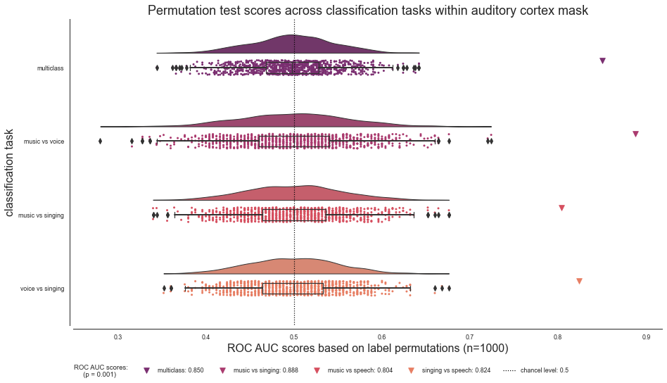
Believe it or not, with that we finished the searchlight analyses portion of the MVPA part of the project. Next, we will focus on ROI decoding, that is repeat the classification tasks from above within a given ROI.
ROI decoding
In contrast to the searchlight analyses the analyses within the ROI decoding portion will not perform a given classification task at multiple locations throughout the auditory cortex by means of a small traveling sphere, but we will run a more “classic” approach. More precisely, we will use the entire voxel pattern of an ROI within the auditory cortex as features within a given classification task. Therefore, we will check if and how well a certain ROI can distinguish between our conditions. If you remember the Auditory Cortex working model section, we actually extract multiple ROIs which we then combined to create our auditory cortex mask. Let’s check them out again before we continue. We will start with defining each via setting its respective path.
HG_left = opj(roi_mask_path, 'tpl-MNI152NLin6Sym_res_02_desc-HGleft_mask.nii.gz')
HG_right = opj(roi_mask_path, 'tpl-MNI152NLin6Sym_res_02_desc-HGright_mask.nii.gz')
PP_left = opj(roi_mask_path, 'tpl-MNI152NLin6Sym_res_02_desc-PPleft_mask.nii.gz')
PP_right = opj(roi_mask_path, 'tpl-MNI152NLin6Sym_res_02_desc-PPright_mask.nii.gz')
PT_left = opj(roi_mask_path, 'tpl-MNI152NLin6Sym_res_02_desc-PTleft_mask.nii.gz')
PT_right = opj(roi_mask_path, 'tpl-MNI152NLin6Sym_res_02_desc-PTright_mask.nii.gz')
aSTG_left = opj(roi_mask_path, 'tpl-MNI152NLin6Sym_res_02_desc-aSTGleft_mask.nii.gz')
aSTG_right = opj(roi_mask_path, 'tpl-MNI152NLin6Sym_res_02_desc-aSTGright_mask.nii.gz')
pSTG_left = opj(roi_mask_path, 'tpl-MNI152NLin6Sym_res_02_desc-pSTGleft_mask.nii.gz')
pSTG_right = opj(roi_mask_path, 'tpl-MNI152NLin6Sym_res_02_desc-pSTGright_mask.nii.gz')
ac_mask = opj(roi_mask_path, 'tpl-MNI152NLin6Sym_res_02_desc-AC_mask.nii.gz')
To ease up further processing steps, we are also going to define two lists: one containing the paths and one containing the names of the ROIs.
list_rois = [HG_left, HG_right, PP_left, PP_right, PT_left, PT_right, aSTG_left, aSTG_right, pSTG_left, pSTG_right]
list_rois_names = ['HG_left', 'HG_right', 'PP_left', 'PP_right', 'PT_left', 'PT_right',
'aSTG_left', 'aSTG_right', 'pSTG_left', 'pSTG_right']
We can now use the same function as in the Auditory Cortex working model section to visualize our ROIs on a template brain:
#suppress contour related warnings
import warnings
warnings.filterwarnings("ignore")
sns.set_style('white')
plt.rcParams["font.family"] = "Arial"
fig=plt.figure(num=None, figsize=(12, 6))
check_ROIs = plot_anat(cut_coords=[-55, -34, 7], figure=fig, draw_cross=False)
check_ROIs.add_contours(HG_left,
colors=[sns.color_palette('cividis', 5)[0]],
filled=True)
check_ROIs.add_contours(PP_left,
colors=[sns.color_palette('cividis', 5)[1]],
filled=True)
check_ROIs.add_contours(PT_left,
colors=[sns.color_palette('cividis', 5)[2]],
filled=True)
check_ROIs.add_contours(aSTG_left,
colors=[sns.color_palette('cividis', 5)[3]],
filled=True)
check_ROIs.add_contours(pSTG_left,
colors=[sns.color_palette('cividis', 5)[4]],
filled=True)
check_ROIs.add_contours(HG_right,
colors=[sns.color_palette('cividis', 5)[0]],
filled=True)
check_ROIs.add_contours(PP_right,
colors=[sns.color_palette('cividis', 5)[1]],
filled=True)
check_ROIs.add_contours(PT_right,
colors=[sns.color_palette('cividis', 5)[2]],
filled=True)
check_ROIs.add_contours(aSTG_right,
colors=[sns.color_palette('cividis', 5)[3]],
filled=True)
check_ROIs.add_contours(pSTG_right,
colors=[sns.color_palette('cividis', 5)[4]],
filled=True)
check_ROIs.add_contours(ac_mask,
levels=[0], colors='black')
mask_legend = [Line2D([0], [0], color='black', lw=4, label='Auditory Cortex\n mask', alpha=0.8)]
first_legend = plt.legend(handles=mask_legend, bbox_to_anchor=(1.5,0.3), loc='right')
plt.gca().add_artist(first_legend)
roi_legend = [Line2D([0], [0], color=sns.color_palette('cividis', 5)[3], lw=4, label='aSTg'),
Line2D([0], [0], color=sns.color_palette('cividis', 5)[1], lw=4, label='PP'),
Line2D([0], [0], color=sns.color_palette('cividis', 5)[0], lw=4, label='HG'),
Line2D([0], [0], color=sns.color_palette('cividis', 5)[2], lw=4, label='PT'),
Line2D([0], [0], color=sns.color_palette('cividis', 5)[4], lw=4, label='pSTG')]
plt.legend(handles=roi_legend, bbox_to_anchor=(1.5,0.5), loc="right", title='ROIs')
plt.text(-215, 90, 'Auditory cortex ROIs',
fontsize=22)
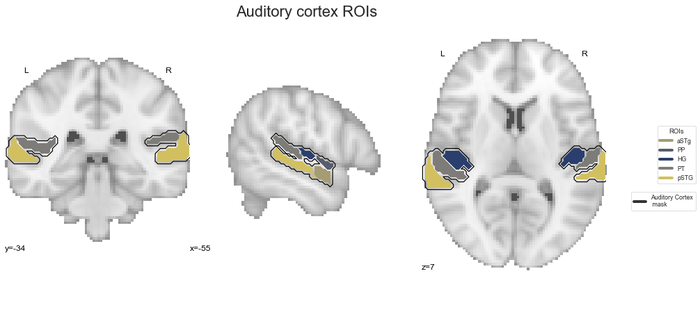
Ah, it looked like that…long time, long time ago… As we remember our ROIs and have prepared them accordingly, we can start with our analyses. Wait what? That fast? How? Well, we spent the better part of this section with defining a lot of functions, including those that we need to run the ROI decoding. If you can not recall that, just go back to the beginning of this section. After setting all analyses parameters we actually defined a function called run_ROI_decoding which brings everything together. Later, we incorporate large parts of that in our run_searchlight_analyses function as well. We can use help() to make sure we initiate the run_ROI_decoding function in the correct manner:
help(run_ROI_decoding)
Help on function run_ROI_decoding in module __main__:
run_ROI_decoding(conditions_cl_task, roi=None, output_path=None)
A small function to ease up the planned decoding tasks.
Providing the conditions to be tested and the ROI they should
be tested in, this function performs the decoding analysis and
the permutation test, as well as saves the outputs to disk.
Parameters
----------
conditions_cl_task : list
List of conditions to be tested
roi : path
Path to ROI conditions should be tested in
output_path : path
Path where results should be stored
The function has 3 input parameters: conditions_cl_task, roi and output_path. As indicated during the definition of the function and comparable to the run_searchlight_analyses function, conditions_cl_task specifies which conditions and thus classification task to be tested and output_path defines where to store results. The roi input parameter is the crucial thing here. In the searchlight analyses we did not set anything, as by default the function will use the auditory cortex mask to extract voxel patterns and run the analyses. Now that we want to evaluate certain ROIs, we need to set this input parameter accordingly. However, as this really the only thing we need to adapt and already have our ROIs set up, we can define a simple for-loop which runs a given classification task for each ROI and stores outputs accordingly. See? It is definitely worth defining a rather complex but solid function. Speaking of which: we need one to visualize the results. Given that we’re now interested in the performance of each ROI, we will define a function which will assign all voxels of an ROI the ROC AUC of that ROI, but only if it is higher than 0.5 and significant as defined by p <= 0.05. Subsequently, all ROIs will be merged together so that we get one image that contains all ROIs with their corresponding ROC AUC scores. The output will be comparable to an atlas, but indicating performance of eachROI.
def plot_roi_decoding_results(conditions_cl_task, output_path=None):
# set classification task name
if len(conditions_cl_task)==2:
task = '%sVS%s' %(conditions_cl_task[0],conditions_cl_task[1])
else:
task = 'multiclass'
# set output path
if output_path is None:
out_path = results_path
else:
out_path = output_path
rois_score = []
for roi in list_rois:
roi_str = roi[roi.rfind('c-')+2:roi.rfind('_mask')]
with open(opj(results_path, 'results/ROI',
"decoding_%s_space-MNI152NLin2009cAsym_desc-permutationscores_mask-%s.json" %(task, roi_str)),
'r' ) as data:
permutation_data = json.load(data)
permutation_scores = permutation_data['permutation_scores']
accuracy = permutation_data['accuracy (ROC AUC)']
p_value = permutation_data['p_value']
roi = nb.load(roi)
roi_data = roi.get_fdata()
roi_data_score = np.zeros_like(roi_data)
if p_value <= 0.05 and accuracy >= 0.5:
roi_data_score[roi_data != 0] = accuracy
rois_score.append(roi_data_score)
rois_score_all = np.sum(np.array(rois_score), axis = 0)
rois_scores_all_image = new_img_like(list_rois[0], rois_score_all)
rois_scores_all_image.to_filename(opj(out_path, 'results/ROI',
"decoding_%s_space-MNI152NLin2009cAsym_desc-permutationscores_mask-ACROIs.nii.gz" %task))
fig=plt.figure(num=None, figsize=(12, 6))
plot_img(rois_scores_all_image, cmap='flare_r', draw_cross=False, cut_coords=[-55, -34, 7], threshold=0.5, colorbar=False,
bg_img=load_mni152_template(), figure=fig)
plt.text(-250,80,'ROI decoding results - %s' %task, fontsize=20)
return rois_score_all, rois_scores_all_image
We will keep the order of classification tasks and start with multiclass.
ROI decoding - multiclass
As in the searchlight analyses, we will at first evaluate if and how well all conditions can be distinguished, but now within each ROI.
for roi in list_rois:
run_ROI_decoding(['music', 'singing', 'voice'], roi=roi)
analyzing the following conditions: ['music' 'singing' 'voice']
[Parallel(n_jobs=3)]: Using backend LokyBackend with 3 concurrent workers.
[Parallel(n_jobs=3)]: Done 44 tasks | elapsed: 4.8s
[Parallel(n_jobs=3)]: Done 194 tasks | elapsed: 15.2s
[Parallel(n_jobs=3)]: Done 444 tasks | elapsed: 34.5s
[Parallel(n_jobs=3)]: Done 794 tasks | elapsed: 1.2min
[Parallel(n_jobs=3)]: Done 1000 out of 1000 | elapsed: 1.5min finished
ROC AUC: 0.3960 / Chance level: 0.5 / p value: 0.9950
saving results to: /data/mvs/derivatives/MVPA/
analyzing the following conditions: ['music' 'singing' 'voice']
[Parallel(n_jobs=3)]: Using backend LokyBackend with 3 concurrent workers.
[Parallel(n_jobs=3)]: Done 44 tasks | elapsed: 3.7s
[Parallel(n_jobs=3)]: Done 194 tasks | elapsed: 13.6s
[Parallel(n_jobs=3)]: Done 444 tasks | elapsed: 27.2s
[Parallel(n_jobs=3)]: Done 794 tasks | elapsed: 44.6s
[Parallel(n_jobs=3)]: Done 1000 out of 1000 | elapsed: 55.4s finished
ROC AUC: 0.4160 / Chance level: 0.5 / p value: 0.9730
saving results to: /data/mvs/derivatives/MVPA/
analyzing the following conditions: ['music' 'singing' 'voice']
[Parallel(n_jobs=3)]: Using backend LokyBackend with 3 concurrent workers.
[Parallel(n_jobs=3)]: Done 44 tasks | elapsed: 2.5s
[Parallel(n_jobs=3)]: Done 194 tasks | elapsed: 13.6s
[Parallel(n_jobs=3)]: Done 444 tasks | elapsed: 28.7s
[Parallel(n_jobs=3)]: Done 794 tasks | elapsed: 49.9s
[Parallel(n_jobs=3)]: Done 1000 out of 1000 | elapsed: 1.0min finished
ROC AUC: 0.6060 / Chance level: 0.5 / p value: 0.0070
saving results to: /data/mvs/derivatives/MVPA/
analyzing the following conditions: ['music' 'singing' 'voice']
[Parallel(n_jobs=3)]: Using backend LokyBackend with 3 concurrent workers.
[Parallel(n_jobs=3)]: Done 82 tasks | elapsed: 6.0s
[Parallel(n_jobs=3)]: Done 382 tasks | elapsed: 31.5s
[Parallel(n_jobs=3)]: Done 882 tasks | elapsed: 1.2min
[Parallel(n_jobs=3)]: Done 995 out of 1000 | elapsed: 1.4min remaining: 0.4s
[Parallel(n_jobs=3)]: Done 1000 out of 1000 | elapsed: 1.4min finished
ROC AUC: 0.6100 / Chance level: 0.5 / p value: 0.0070
saving results to: /data/mvs/derivatives/MVPA/
analyzing the following conditions: ['music' 'singing' 'voice']
[Parallel(n_jobs=3)]: Using backend LokyBackend with 3 concurrent workers.
[Parallel(n_jobs=3)]: Done 44 tasks | elapsed: 4.5s
[Parallel(n_jobs=3)]: Done 194 tasks | elapsed: 18.1s
[Parallel(n_jobs=3)]: Done 444 tasks | elapsed: 39.8s
[Parallel(n_jobs=3)]: Done 794 tasks | elapsed: 1.1min
[Parallel(n_jobs=3)]: Done 1000 out of 1000 | elapsed: 1.4min finished
ROC AUC: 0.7300 / Chance level: 0.5 / p value: 0.0010
saving results to: /data/mvs/derivatives/MVPA/
analyzing the following conditions: ['music' 'singing' 'voice']
[Parallel(n_jobs=3)]: Using backend LokyBackend with 3 concurrent workers.
[Parallel(n_jobs=3)]: Done 44 tasks | elapsed: 3.3s
[Parallel(n_jobs=3)]: Done 194 tasks | elapsed: 15.4s
[Parallel(n_jobs=3)]: Done 444 tasks | elapsed: 37.1s
[Parallel(n_jobs=3)]: Done 794 tasks | elapsed: 1.1min
[Parallel(n_jobs=3)]: Done 1000 out of 1000 | elapsed: 1.3min finished
ROC AUC: 0.3130 / Chance level: 0.5 / p value: 1.0000
saving results to: /data/mvs/derivatives/MVPA/
analyzing the following conditions: ['music' 'singing' 'voice']
[Parallel(n_jobs=3)]: Using backend LokyBackend with 3 concurrent workers.
[Parallel(n_jobs=3)]: Done 44 tasks | elapsed: 4.1s
[Parallel(n_jobs=3)]: Done 194 tasks | elapsed: 17.3s
[Parallel(n_jobs=3)]: Done 444 tasks | elapsed: 39.6s
[Parallel(n_jobs=3)]: Done 794 tasks | elapsed: 1.1min
[Parallel(n_jobs=3)]: Done 1000 out of 1000 | elapsed: 1.3min finished
ROC AUC: 0.7400 / Chance level: 0.5 / p value: 0.0010
saving results to: /data/mvs/derivatives/MVPA/
analyzing the following conditions: ['music' 'singing' 'voice']
[Parallel(n_jobs=3)]: Using backend LokyBackend with 3 concurrent workers.
[Parallel(n_jobs=3)]: Done 44 tasks | elapsed: 3.1s
[Parallel(n_jobs=3)]: Done 194 tasks | elapsed: 14.1s
[Parallel(n_jobs=3)]: Done 444 tasks | elapsed: 35.4s
[Parallel(n_jobs=3)]: Done 794 tasks | elapsed: 1.0min
[Parallel(n_jobs=3)]: Done 1000 out of 1000 | elapsed: 1.2min finished
ROC AUC: 0.8440 / Chance level: 0.5 / p value: 0.0010
saving results to: /data/mvs/derivatives/MVPA/
analyzing the following conditions: ['music' 'singing' 'voice']
[Parallel(n_jobs=3)]: Using backend LokyBackend with 3 concurrent workers.
[Parallel(n_jobs=3)]: Done 44 tasks | elapsed: 4.5s
[Parallel(n_jobs=3)]: Done 194 tasks | elapsed: 19.7s
[Parallel(n_jobs=3)]: Done 444 tasks | elapsed: 44.4s
[Parallel(n_jobs=3)]: Done 794 tasks | elapsed: 1.3min
[Parallel(n_jobs=3)]: Done 1000 out of 1000 | elapsed: 1.7min finished
ROC AUC: 0.8160 / Chance level: 0.5 / p value: 0.0010
saving results to: /data/mvs/derivatives/MVPA/
analyzing the following conditions: ['music' 'singing' 'voice']
[Parallel(n_jobs=3)]: Using backend LokyBackend with 3 concurrent workers.
[Parallel(n_jobs=3)]: Done 44 tasks | elapsed: 6.4s
[Parallel(n_jobs=3)]: Done 194 tasks | elapsed: 24.0s
[Parallel(n_jobs=3)]: Done 444 tasks | elapsed: 52.6s
[Parallel(n_jobs=3)]: Done 794 tasks | elapsed: 1.5min
ROC AUC: 0.7680 / Chance level: 0.5 / p value: 0.0010
saving results to: /data/mvs/derivatives/MVPA/
[Parallel(n_jobs=3)]: Done 1000 out of 1000 | elapsed: 1.9min finished
We already got a glimpse of the output, but let’s visualize it:
scores, scores_image = plot_roi_decoding_results(['music', 'singing', 'voice'])
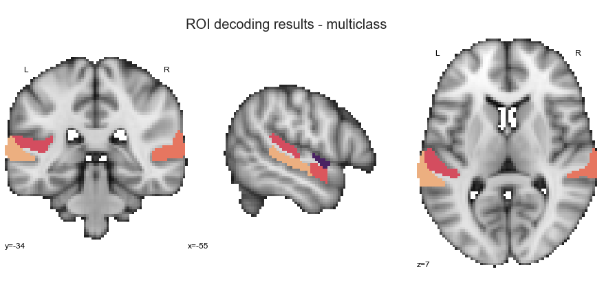
We also generate an interactive surface plot to some exploration:
view_img_on_surf(scores_image, cmap='flare_r', threshold=0.001, symmetric_cmap=False)
Please note that for example HG right is missing as its performance was below 0.5 and additionally not significant.
ROI decoding - music vs. voice
Next on the list is the music vs. voice classification task.
for roi in list_rois:
run_ROI_decoding(['music', 'voice'], roi=roi)
analyzing the following conditions: ['music' 'voice']
[Parallel(n_jobs=3)]: Using backend LokyBackend with 3 concurrent workers.
[Parallel(n_jobs=3)]: Done 92 tasks | elapsed: 3.2s
[Parallel(n_jobs=3)]: Done 692 tasks | elapsed: 13.5s
[Parallel(n_jobs=3)]: Done 1000 out of 1000 | elapsed: 18.8s finished
[Parallel(n_jobs=3)]: Using backend LokyBackend with 3 concurrent workers.
ROC AUC: 0.6800 / Chance level: 0.50 / p value: 0.0020
saving results to: /data/mvs/derivatives/MVPA/
analyzing the following conditions: ['music' 'voice']
[Parallel(n_jobs=3)]: Done 146 tasks | elapsed: 2.5s
[Parallel(n_jobs=3)]: Done 746 tasks | elapsed: 11.6s
[Parallel(n_jobs=3)]: Done 1000 out of 1000 | elapsed: 15.3s finished
[Parallel(n_jobs=3)]: Using backend LokyBackend with 3 concurrent workers.
ROC AUC: 0.5800 / Chance level: 0.50 / p value: 0.0629
saving results to: /data/mvs/derivatives/MVPA/
analyzing the following conditions: ['music' 'voice']
[Parallel(n_jobs=3)]: Done 146 tasks | elapsed: 2.5s
[Parallel(n_jobs=3)]: Done 746 tasks | elapsed: 12.3s
[Parallel(n_jobs=3)]: Done 1000 out of 1000 | elapsed: 17.9s finished
[Parallel(n_jobs=3)]: Using backend LokyBackend with 3 concurrent workers.
ROC AUC: 0.6960 / Chance level: 0.50 / p value: 0.0020
saving results to: /data/mvs/derivatives/MVPA/
analyzing the following conditions: ['music' 'voice']
[Parallel(n_jobs=3)]: Done 82 tasks | elapsed: 3.4s
[Parallel(n_jobs=3)]: Done 382 tasks | elapsed: 17.2s
[Parallel(n_jobs=3)]: Done 882 tasks | elapsed: 27.9s
[Parallel(n_jobs=3)]: Done 995 out of 1000 | elapsed: 30.2s remaining: 0.2s
[Parallel(n_jobs=3)]: Done 1000 out of 1000 | elapsed: 30.3s finished
[Parallel(n_jobs=3)]: Using backend LokyBackend with 3 concurrent workers.
ROC AUC: 0.7200 / Chance level: 0.50 / p value: 0.0010
saving results to: /data/mvs/derivatives/MVPA/
analyzing the following conditions: ['music' 'voice']
[Parallel(n_jobs=3)]: Done 146 tasks | elapsed: 3.6s
[Parallel(n_jobs=3)]: Done 746 tasks | elapsed: 16.6s
[Parallel(n_jobs=3)]: Done 1000 out of 1000 | elapsed: 22.3s finished
[Parallel(n_jobs=3)]: Using backend LokyBackend with 3 concurrent workers.
ROC AUC: 0.7880 / Chance level: 0.50 / p value: 0.0010
saving results to: /data/mvs/derivatives/MVPA/
analyzing the following conditions: ['music' 'voice']
[Parallel(n_jobs=3)]: Done 146 tasks | elapsed: 3.0s
[Parallel(n_jobs=3)]: Done 746 tasks | elapsed: 15.5s
[Parallel(n_jobs=3)]: Done 1000 out of 1000 | elapsed: 20.6s finished
[Parallel(n_jobs=3)]: Using backend LokyBackend with 3 concurrent workers.
ROC AUC: 0.6680 / Chance level: 0.50 / p value: 0.0010
saving results to: /data/mvs/derivatives/MVPA/
analyzing the following conditions: ['music' 'voice']
[Parallel(n_jobs=3)]: Done 146 tasks | elapsed: 2.9s
[Parallel(n_jobs=3)]: Done 746 tasks | elapsed: 14.9s
[Parallel(n_jobs=3)]: Done 1000 out of 1000 | elapsed: 19.6s finished
[Parallel(n_jobs=3)]: Using backend LokyBackend with 3 concurrent workers.
ROC AUC: 0.9040 / Chance level: 0.50 / p value: 0.0010
saving results to: /data/mvs/derivatives/MVPA/
analyzing the following conditions: ['music' 'voice']
[Parallel(n_jobs=3)]: Done 146 tasks | elapsed: 3.8s
[Parallel(n_jobs=3)]: Done 746 tasks | elapsed: 16.2s
[Parallel(n_jobs=3)]: Done 1000 out of 1000 | elapsed: 22.5s finished
[Parallel(n_jobs=3)]: Using backend LokyBackend with 3 concurrent workers.
ROC AUC: 0.8560 / Chance level: 0.50 / p value: 0.0010
saving results to: /data/mvs/derivatives/MVPA/
analyzing the following conditions: ['music' 'voice']
[Parallel(n_jobs=3)]: Done 146 tasks | elapsed: 3.2s
[Parallel(n_jobs=3)]: Done 746 tasks | elapsed: 21.1s
[Parallel(n_jobs=3)]: Done 1000 out of 1000 | elapsed: 27.2s finished
[Parallel(n_jobs=3)]: Using backend LokyBackend with 3 concurrent workers.
ROC AUC: 0.8760 / Chance level: 0.50 / p value: 0.0010
saving results to: /data/mvs/derivatives/MVPA/
analyzing the following conditions: ['music' 'voice']
[Parallel(n_jobs=3)]: Done 146 tasks | elapsed: 3.2s
[Parallel(n_jobs=3)]: Done 746 tasks | elapsed: 14.8s
ROC AUC: 0.8160 / Chance level: 0.50 / p value: 0.0010
saving results to: /data/mvs/derivatives/MVPA/
[Parallel(n_jobs=3)]: Done 1000 out of 1000 | elapsed: 20.2s finished
How do the results look like?
scores, scores_image = plot_roi_decoding_results(['music', 'voice'])
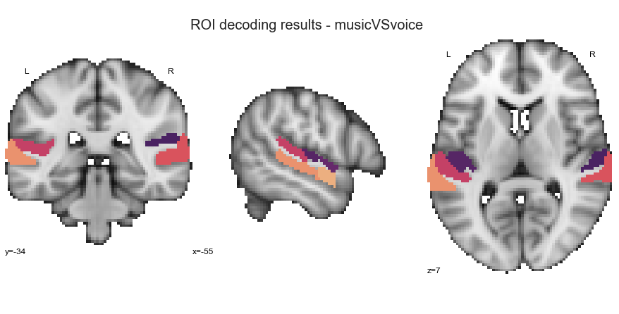
Here iss the interactive surface plot version:
view_img_on_surf(scores_image, cmap='flare_r', threshold=0.001, symmetric_cmap=False)
Decoding analyses - music vs. singing
Let’s see how the ROIs perform for the music vs. singing classification task:
for roi in list_rois:
run_ROI_decoding(['music', 'singing'], roi=roi)
[Parallel(n_jobs=3)]: Using backend LokyBackend with 3 concurrent workers.
analyzing the following conditions: ['music' 'singing']
[Parallel(n_jobs=3)]: Done 146 tasks | elapsed: 2.5s
[Parallel(n_jobs=3)]: Done 746 tasks | elapsed: 13.3s
[Parallel(n_jobs=3)]: Done 1000 out of 1000 | elapsed: 17.4s finished
[Parallel(n_jobs=3)]: Using backend LokyBackend with 3 concurrent workers.
ROC AUC: 0.5800 / Chance level: 0.50 / p value: 0.0340
saving results to: /data/mvs/derivatives/MVPA/
analyzing the following conditions: ['music' 'singing']
[Parallel(n_jobs=3)]: Done 146 tasks | elapsed: 2.4s
[Parallel(n_jobs=3)]: Done 746 tasks | elapsed: 11.9s
[Parallel(n_jobs=3)]: Done 1000 out of 1000 | elapsed: 15.6s finished
[Parallel(n_jobs=3)]: Using backend LokyBackend with 3 concurrent workers.
ROC AUC: 0.5560 / Chance level: 0.50 / p value: 0.1499
saving results to: /data/mvs/derivatives/MVPA/
analyzing the following conditions: ['music' 'singing']
[Parallel(n_jobs=3)]: Done 146 tasks | elapsed: 2.5s
[Parallel(n_jobs=3)]: Done 746 tasks | elapsed: 11.9s
[Parallel(n_jobs=3)]: Done 1000 out of 1000 | elapsed: 16.6s finished
[Parallel(n_jobs=3)]: Using backend LokyBackend with 3 concurrent workers.
ROC AUC: 0.6680 / Chance level: 0.50 / p value: 0.0030
saving results to: /data/mvs/derivatives/MVPA/
analyzing the following conditions: ['music' 'singing']
[Parallel(n_jobs=3)]: Done 146 tasks | elapsed: 3.6s
[Parallel(n_jobs=3)]: Done 746 tasks | elapsed: 17.7s
[Parallel(n_jobs=3)]: Done 1000 out of 1000 | elapsed: 21.7s finished
[Parallel(n_jobs=3)]: Using backend LokyBackend with 3 concurrent workers.
ROC AUC: 0.7280 / Chance level: 0.50 / p value: 0.0010
saving results to: /data/mvs/derivatives/MVPA/
analyzing the following conditions: ['music' 'singing']
[Parallel(n_jobs=3)]: Done 92 tasks | elapsed: 1.9s
[Parallel(n_jobs=3)]: Done 692 tasks | elapsed: 14.8s
[Parallel(n_jobs=3)]: Done 1000 out of 1000 | elapsed: 21.1s finished
[Parallel(n_jobs=3)]: Using backend LokyBackend with 3 concurrent workers.
ROC AUC: 0.6840 / Chance level: 0.50 / p value: 0.0010
saving results to: /data/mvs/derivatives/MVPA/
analyzing the following conditions: ['music' 'singing']
[Parallel(n_jobs=3)]: Done 146 tasks | elapsed: 4.9s
[Parallel(n_jobs=3)]: Done 746 tasks | elapsed: 20.8s
[Parallel(n_jobs=3)]: Done 1000 out of 1000 | elapsed: 26.3s finished
[Parallel(n_jobs=3)]: Using backend LokyBackend with 3 concurrent workers.
ROC AUC: 0.6680 / Chance level: 0.50 / p value: 0.0010
saving results to: /data/mvs/derivatives/MVPA/
analyzing the following conditions: ['music' 'singing']
[Parallel(n_jobs=3)]: Done 146 tasks | elapsed: 2.9s
[Parallel(n_jobs=3)]: Done 746 tasks | elapsed: 13.8s
[Parallel(n_jobs=3)]: Done 1000 out of 1000 | elapsed: 18.9s finished
[Parallel(n_jobs=3)]: Using backend LokyBackend with 3 concurrent workers.
ROC AUC: 0.6760 / Chance level: 0.50 / p value: 0.0050
saving results to: /data/mvs/derivatives/MVPA/
analyzing the following conditions: ['music' 'singing']
[Parallel(n_jobs=3)]: Done 146 tasks | elapsed: 3.2s
[Parallel(n_jobs=3)]: Done 746 tasks | elapsed: 14.8s
[Parallel(n_jobs=3)]: Done 1000 out of 1000 | elapsed: 19.3s finished
[Parallel(n_jobs=3)]: Using backend LokyBackend with 3 concurrent workers.
ROC AUC: 0.8000 / Chance level: 0.50 / p value: 0.0010
saving results to: /data/mvs/derivatives/MVPA/
analyzing the following conditions: ['music' 'singing']
[Parallel(n_jobs=3)]: Done 146 tasks | elapsed: 3.4s
[Parallel(n_jobs=3)]: Done 746 tasks | elapsed: 16.8s
[Parallel(n_jobs=3)]: Done 1000 out of 1000 | elapsed: 22.5s finished
[Parallel(n_jobs=3)]: Using backend LokyBackend with 3 concurrent workers.
ROC AUC: 0.7440 / Chance level: 0.50 / p value: 0.0010
saving results to: /data/mvs/derivatives/MVPA/
analyzing the following conditions: ['music' 'singing']
[Parallel(n_jobs=3)]: Done 146 tasks | elapsed: 3.4s
[Parallel(n_jobs=3)]: Done 746 tasks | elapsed: 18.3s
ROC AUC: 0.7120 / Chance level: 0.50 / p value: 0.0010
saving results to: /data/mvs/derivatives/MVPA/
[Parallel(n_jobs=3)]: Done 1000 out of 1000 | elapsed: 23.0s finished
As done before, we can investigate the results using our visualization function in the static volume version:
scores, scores_image = plot_roi_decoding_results(['music', 'singing'])
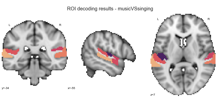
and the interactive surface version:
view_img_on_surf(scores_image, cmap='flare_r', threshold=0.001, symmetric_cmap=False)
ROI decoding - voice vs. singing
Last, but not least: the voice vs. singing classification task.
for roi in list_rois:
run_ROI_decoding(['voice', 'singing'], roi=roi)
[Parallel(n_jobs=3)]: Using backend LokyBackend with 3 concurrent workers.
analyzing the following conditions: ['singing' 'voice']
[Parallel(n_jobs=3)]: Done 146 tasks | elapsed: 2.2s
[Parallel(n_jobs=3)]: Done 746 tasks | elapsed: 12.5s
[Parallel(n_jobs=3)]: Done 1000 out of 1000 | elapsed: 16.9s finished
[Parallel(n_jobs=3)]: Using backend LokyBackend with 3 concurrent workers.
ROC AUC: 0.5800 / Chance level: 0.50 / p value: 0.0470
saving results to: /data/mvs/derivatives/MVPA/
analyzing the following conditions: ['singing' 'voice']
[Parallel(n_jobs=3)]: Done 146 tasks | elapsed: 2.2s
[Parallel(n_jobs=3)]: Done 746 tasks | elapsed: 15.5s
[Parallel(n_jobs=3)]: Done 1000 out of 1000 | elapsed: 23.3s finished
[Parallel(n_jobs=3)]: Using backend LokyBackend with 3 concurrent workers.
ROC AUC: 0.5680 / Chance level: 0.50 / p value: 0.1109
saving results to: /data/mvs/derivatives/MVPA/
analyzing the following conditions: ['singing' 'voice']
[Parallel(n_jobs=3)]: Done 146 tasks | elapsed: 4.1s
[Parallel(n_jobs=3)]: Done 746 tasks | elapsed: 14.3s
[Parallel(n_jobs=3)]: Done 1000 out of 1000 | elapsed: 18.3s finished
[Parallel(n_jobs=3)]: Using backend LokyBackend with 3 concurrent workers.
ROC AUC: 0.6520 / Chance level: 0.50 / p value: 0.0010
saving results to: /data/mvs/derivatives/MVPA/
analyzing the following conditions: ['singing' 'voice']
[Parallel(n_jobs=3)]: Done 146 tasks | elapsed: 2.6s
[Parallel(n_jobs=3)]: Done 746 tasks | elapsed: 12.1s
[Parallel(n_jobs=3)]: Done 1000 out of 1000 | elapsed: 15.7s finished
[Parallel(n_jobs=3)]: Using backend LokyBackend with 3 concurrent workers.
ROC AUC: 0.5960 / Chance level: 0.50 / p value: 0.0330
saving results to: /data/mvs/derivatives/MVPA/
analyzing the following conditions: ['singing' 'voice']
[Parallel(n_jobs=3)]: Done 146 tasks | elapsed: 2.6s
[Parallel(n_jobs=3)]: Done 746 tasks | elapsed: 13.1s
[Parallel(n_jobs=3)]: Done 1000 out of 1000 | elapsed: 17.1s finished
[Parallel(n_jobs=3)]: Using backend LokyBackend with 3 concurrent workers.
ROC AUC: 0.6640 / Chance level: 0.50 / p value: 0.0020
saving results to: /data/mvs/derivatives/MVPA/
analyzing the following conditions: ['singing' 'voice']
[Parallel(n_jobs=3)]: Done 146 tasks | elapsed: 2.7s
[Parallel(n_jobs=3)]: Done 746 tasks | elapsed: 12.0s
[Parallel(n_jobs=3)]: Done 1000 out of 1000 | elapsed: 15.9s finished
[Parallel(n_jobs=3)]: Using backend LokyBackend with 3 concurrent workers.
ROC AUC: 0.5840 / Chance level: 0.50 / p value: 0.0190
saving results to: /data/mvs/derivatives/MVPA/
analyzing the following conditions: ['singing' 'voice']
[Parallel(n_jobs=3)]: Done 146 tasks | elapsed: 2.2s
[Parallel(n_jobs=3)]: Done 746 tasks | elapsed: 10.9s
[Parallel(n_jobs=3)]: Done 1000 out of 1000 | elapsed: 14.2s finished
[Parallel(n_jobs=3)]: Using backend LokyBackend with 3 concurrent workers.
ROC AUC: 0.7880 / Chance level: 0.50 / p value: 0.0010
saving results to: /data/mvs/derivatives/MVPA/
analyzing the following conditions: ['singing' 'voice']
[Parallel(n_jobs=3)]: Done 146 tasks | elapsed: 2.2s
[Parallel(n_jobs=3)]: Done 746 tasks | elapsed: 10.6s
[Parallel(n_jobs=3)]: Done 1000 out of 1000 | elapsed: 14.1s finished
[Parallel(n_jobs=3)]: Using backend LokyBackend with 3 concurrent workers.
ROC AUC: 0.7720 / Chance level: 0.50 / p value: 0.0010
saving results to: /data/mvs/derivatives/MVPA/
analyzing the following conditions: ['singing' 'voice']
[Parallel(n_jobs=3)]: Done 146 tasks | elapsed: 3.2s
[Parallel(n_jobs=3)]: Done 746 tasks | elapsed: 15.3s
[Parallel(n_jobs=3)]: Done 1000 out of 1000 | elapsed: 20.2s finished
[Parallel(n_jobs=3)]: Using backend LokyBackend with 3 concurrent workers.
ROC AUC: 0.7560 / Chance level: 0.50 / p value: 0.0010
saving results to: /data/mvs/derivatives/MVPA/
analyzing the following conditions: ['singing' 'voice']
[Parallel(n_jobs=3)]: Done 146 tasks | elapsed: 3.0s
[Parallel(n_jobs=3)]: Done 746 tasks | elapsed: 15.3s
ROC AUC: 0.7160 / Chance level: 0.50 / p value: 0.0010
saving results to: /data/mvs/derivatives/MVPA/
[Parallel(n_jobs=3)]: Done 1000 out of 1000 | elapsed: 21.6s finished
And again: the outcomes visualized as usual.
scores, scores_image = plot_roi_decoding_results(['voice', 'singing'])
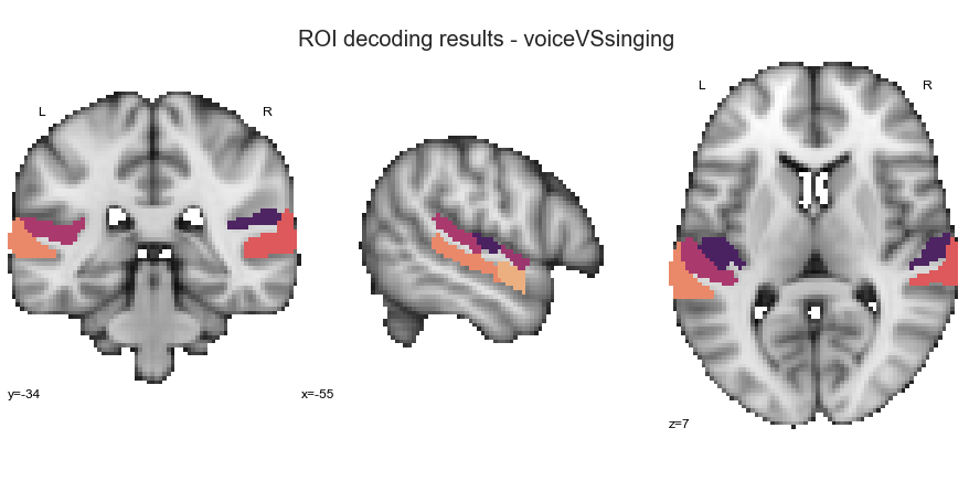
And one last time, the interactive surface version:
view_img_on_surf(scores_image, cmap='flare_r', threshold=0.001, symmetric_cmap=False)
This already concludes the end of the ROI decoding analyses, at least concerning the classification tasks introduced in the beginning. What follows is the final portion of the conducted complementary MVPA.
ROI decoding - condition specific
In order to investigate the extent to which voxel patterns in the audicory cortex carry information necessary to distinguish the tested conditions, we specified the same four classification tasks: multiclass, music vs. voice, music vs. singing and voice vs. singing. We conducted the corresponding analyses at two scales: the entire auditory cortex by means of searchlight analyses and within certain ROIs reflection different regions of the auditory cortex. Being complementary in nature and aiming to provide as much insight as possible, we will run a third type of MVPA within which we will focus on ROI voxel pattern again, but now focusing on a single condition instead of a distinction between conditions. This is motivated by obtaining a single value for an analyses involving two or three conditions in the previous steps, thus not entailing information on single conditions and if one is driving the classification more than the other. Luckily, we already have everything we need to do this and also don’t need to define a function, as we will run this only once. We can simply use the parts we set up in the beginning and pack everything in a for-loop that runs the steps for each ROI. The only difference is that we define a single decoding target. To do that we just need to get the unique conditions from our decoding information “conditions”:
conditions_unique = conditions.unique()
conditions_unique
array(['music', 'singing', 'voice'], dtype=object)
We get music, singing and voice which is correct. Next, we will define a few empty dictionaries to save our results to, including the ROC AUC score, permutation score and p values.
mask_scores = {}
mask_chance_scores = {}
mask_scores_p = {}
And we are good to go. What follows is a small for-loop that runs the analyses for each ROI and each condition. ROC AUC scores and permutation scores are computed as before:
for roi_name,roi in zip(list_rois_names, list_rois):
print("Working on mask %s" %roi_name)
masker = NiftiMasker(mask_img=roi)
img_data = masker.fit_transform(con_images)
mask_scores[roi_name] = {}
mask_scores_p[roi_name] = {}
for condition in conditions_unique:
print("Processing %s %s" % (roi_name, condition))
classification_target = (conditions == condition)
mask_scores[roi_name][condition] = cross_val_score(pipeline, img_data,
classification_target,
cv=cv, scoring="roc_auc",
groups=participants
)
mask_scores_p[roi_name][condition] = permutation_test_score(pipeline, img_data,
classification_target,
cv=cv, scoring="roc_auc",
groups=participants,
n_permutations=1000, n_jobs=3
)
print("Scores: %1.2f +- %1.2f, p value: %1.2f" % (
mask_scores[roi_name][condition].mean(),
mask_scores[roi_name][condition].std(),
mask_scores_p[roi_name][condition][2]))
Working on mask HG_left
Processing HG_left music
Scores: 0.65 +- 0.09, p value: 0.00
Processing HG_left singing
Scores: 0.59 +- 0.07, p value: 0.01
Processing HG_left voice
Scores: 0.61 +- 0.08, p value: 0.01
Working on mask HG_right
Processing HG_right music
Scores: 0.58 +- 0.03, p value: 0.03
Processing HG_right singing
Scores: 0.55 +- 0.06, p value: 0.09
Processing HG_right voice
Scores: 0.58 +- 0.10, p value: 0.04
Working on mask PP_left
Processing PP_left music
Scores: 0.67 +- 0.12, p value: 0.00
Processing PP_left singing
Scores: 0.58 +- 0.05, p value: 0.04
Processing PP_left voice
Scores: 0.71 +- 0.08, p value: 0.00
Working on mask PP_right
Processing PP_right music
Scores: 0.73 +- 0.07, p value: 0.00
Processing PP_right singing
Scores: 0.62 +- 0.07, p value: 0.00
Processing PP_right voice
Scores: 0.64 +- 0.09, p value: 0.00
Working on mask PT_left
Processing PT_left music
Scores: 0.73 +- 0.09, p value: 0.00
Processing PT_left singing
Scores: 0.51 +- 0.03, p value: 0.38
Processing PT_left voice
Scores: 0.76 +- 0.07, p value: 0.00
Working on mask PT_right
Processing PT_right music
Scores: 0.72 +- 0.12, p value: 0.00
Processing PT_right singing
Scores: 0.52 +- 0.03, p value: 0.28
Processing PT_right voice
Scores: 0.65 +- 0.04, p value: 0.00
Working on mask aSTG_left
Processing aSTG_left music
Scores: 0.79 +- 0.09, p value: 0.00
Processing aSTG_left singing
Scores: 0.53 +- 0.04, p value: 0.25
Processing aSTG_left voice
Scores: 0.86 +- 0.06, p value: 0.00
Working on mask aSTG_right
Processing aSTG_right music
Scores: 0.84 +- 0.11, p value: 0.00
Processing aSTG_right singing
Scores: 0.54 +- 0.04, p value: 0.20
Processing aSTG_right voice
Scores: 0.81 +- 0.07, p value: 0.00
Working on mask pSTG_left
Processing pSTG_left music
Scores: 0.82 +- 0.10, p value: 0.00
Processing pSTG_left singing
Scores: 0.57 +- 0.06, p value: 0.09
Processing pSTG_left voice
Scores: 0.81 +- 0.10, p value: 0.00
Working on mask pSTG_right
Processing pSTG_right music
Scores: 0.77 +- 0.10, p value: 0.00
Processing pSTG_right singing
Scores: 0.63 +- 0.05, p value: 0.00
Processing pSTG_right voice
Scores: 0.79 +- 0.11, p value: 0.00
That was…a lot. Let’s bring the results into a form that eases up saving, handling and plotting.
ROI_decoding_scores = {}
for roi_name in list_rois_names:
ROI_decoding_scores[roi_name] = {}
for condition in conditions_unique:
print("Processing %s %s" % (roi_name, condition))
ROI_decoding_scores[roi_name][condition] = {}
ROI_decoding_scores[roi_name][condition]['ROC_AUC'] = mask_scores_p[roi_name][condition][0]
ROI_decoding_scores[roi_name][condition]['permutation scores'] = list(mask_scores_p[roi_name][condition][1])
ROI_decoding_scores[roi_name][condition]['p value'] = mask_scores_p[roi_name][condition][2]
Processing HG_left music
Processing HG_left singing
Processing HG_left voice
Processing HG_right music
Processing HG_right singing
Processing HG_right voice
Processing PP_left music
Processing PP_left singing
Processing PP_left voice
Processing PP_right music
Processing PP_right singing
Processing PP_right voice
Processing PT_left music
Processing PT_left singing
Processing PT_left voice
Processing PT_right music
Processing PT_right singing
Processing PT_right voice
Processing aSTG_left music
Processing aSTG_left singing
Processing aSTG_left voice
Processing aSTG_right music
Processing aSTG_right singing
Processing aSTG_right voice
Processing pSTG_left music
Processing pSTG_left singing
Processing pSTG_left voice
Processing pSTG_right music
Processing pSTG_right singing
Processing pSTG_right voice
What we have now is a dictionary which contains the ROC AUC score, permutation test scores and p value for each classification target (i.e. condition) and ROI. In this form, we can save it:
json.dump(ROI_decoding_scores, open(opj(results_path, 'results/ROI',
"decoding_AllConditions_space-MNI152NLin2009cAsym_desc-permutationscores_ROIs.json"),
'w' ))
In order to visualize such an amount of information in a meaningful and understandable way, we have to think more than twice…We all know that bar plots are not the way to go in the majority of cases and the same holds true for the one at hand, especially as we the ROC AUC scores are single data points. However, setting up a plot within which each ROC AUC score per condition and ROI is visualized as a bar, with the mean and std of the permutation test scores put on top of that might actually do the trick. In more detail, we plot the results based on hemisphere and ROI with the condition specific outcomes ordered accordingly. Given that this will result in a clean and “minimal” plot and because it is important, we will also markers that indicate the significance of a given outcome. What follows is a lot of code, but as said before: graphics are important.
cmap = plt.cm.get_cmap('Set2')
music_color = cmap(0.3)
voice_color = cmap(0.2)
singing_color = cmap(0.0)
sns.set_context('paper')
sns.set_style('whitegrid')
plt.rcParams["font.family"] = "Arial"
import numpy as np
import matplotlib.pyplot as plt
plt.figure(figsize=(10,6))
names_rois = ['STGp', 'PT', 'HG', 'PP', 'STGa']
names_rois_left = ['pSTG_left', 'PT_left','HG_left', 'PP_left', 'aSTG_left']
names_rois_right = ['pSTG_right', 'PT_right', 'HG_right', 'PP_right', 'aSTG_right']
plt.subplot(1, 2, 1)
tick_position = np.arange(len(names_rois))
plt.yticks([tick_position + 0.3 for tick_position in tick_position], names_rois)
color_list = [music_color, singing_color, voice_color]
for color, condition in zip(color_list, ['music', 'singing', 'voice']):
score_means = [ROI_decoding_scores[mask_name][condition]['ROC_AUC'] for mask_name in names_rois_left]
marker_pos = [ROI_decoding_scores[mask_name][condition]['ROC_AUC'] + 0.01 for mask_name in names_rois_left]
plt.barh(tick_position, score_means, label=condition, color=color,height=.25) #
pvalue = [ROI_decoding_scores[mask_name][condition]['p value'] for mask_name in names_rois_left]
plt.xlim(0.4, 1)
plt.box(False)
plt.gca().invert_xaxis()
plt.yticks([])
score_perm = [np.mean(ROI_decoding_scores[mask_name][condition]['permutation scores'])
for mask_name in names_rois_left]
std_perm = [np.std(ROI_decoding_scores[mask_name][condition]['permutation scores'])
for mask_name in names_rois_left]
plt.barh(tick_position, score_perm, edgecolor='k', facecolor='none',height=.25, xerr=std_perm)
for n, p in enumerate(pvalue):
if p < 0.05 and p > 0.01:
plt.scatter(marker_pos[n],tick_position[n],marker='*', color='black')
elif p < 0.01:
plt.scatter(marker_pos[n],tick_position[n],marker='d', color='black')
tick_position = tick_position + 0.3
plt.subplots_adjust(wspace=0.3)
plt.ylabel('auditory pathway ROIs', fontsize=15)
plt.subplot(1, 2, 2)
tick_position = np.arange(len(names_rois))
plt.yticks([tick_position + 0.3 for tick_position in tick_position], names_rois)
color_list = [music_color, singing_color, voice_color]
for color, condition in zip(color_list, ['music', 'singing', 'voice']):
score_means = [ROI_decoding_scores[mask_name][condition]['ROC_AUC'] for mask_name in names_rois_right]
marker_pos = [ROI_decoding_scores[mask_name][condition]['ROC_AUC'] + 0.01 for mask_name in names_rois_right]
plt.barh(tick_position, score_means, label=condition, color=color,height=.25) #
pvalue = [ROI_decoding_scores[mask_name][condition]['p value'] for mask_name in names_rois_right]
plt.xlim(0.4, 1)
plt.box(False)
plt.yticks([])
score_perm = [np.mean(ROI_decoding_scores[mask_name][condition]['permutation scores'])
for mask_name in names_rois_right]
std_perm = [np.std(ROI_decoding_scores[mask_name][condition]['permutation scores'])
for mask_name in names_rois_right]
plt.barh(tick_position, score_perm, edgecolor='k', facecolor='none',height=.25, xerr=std_perm)
for n, p in enumerate(pvalue):
if p < 0.05 and p > 0.01:
plt.scatter(marker_pos[n],tick_position[n],marker='*', color='black')
elif p < 0.01:
plt.scatter(marker_pos[n],tick_position[n],marker='d', color='black')
tick_position = tick_position + 0.3
plt.text(0.305, 4.3, 'aSTG', horizontalalignment='center',verticalalignment='center', fontsize=15)
plt.text(0.305, 3.3, 'PP', horizontalalignment='center',verticalalignment='center', fontsize=15)
plt.text(0.305, 2.3, 'HG', horizontalalignment='center',verticalalignment='center', fontsize=15)
plt.text(0.305, 1.3, 'PT', horizontalalignment='center',verticalalignment='center', fontsize=15)
plt.text(0.305, 0.3, 'pSTG', horizontalalignment='center',verticalalignment='center', fontsize=15)
plt.text(0.305, -1.1, 'ROC AUC score', horizontalalignment='center',verticalalignment='center', fontsize=15)
plt.text(-0.03, 5.2, 'left hemisphere', horizontalalignment='center',verticalalignment='center', fontsize=15)
plt.text(0.65, 5.2, 'right hemisphere', horizontalalignment='center',verticalalignment='center', fontsize=15)
roi_legend = [Line2D([0], [0], color=colors.to_hex(voice_color), lw=4, label='voice'),
Line2D([0], [0], color='black', lw=4, label='mean/std 1000 permutations'),
Line2D([0], [0], color=colors.to_hex(singing_color), lw=4, label='singing'),
Line2D([0], [0], marker='d', color='w', markerfacecolor='black',
label='p < 0.01', markersize=10),
Line2D([0], [0], color=colors.to_hex(music_color), lw=4, label='music'),
Line2D([0], [0], marker='*', color='w', markerfacecolor='black',
label='p < 0.05 & p > 0.01', markersize=12)
]
plt.legend(handles=roi_legend, bbox_to_anchor=(-0.15, -0.33), fontsize=12, ncol=3, loc="lower center", frameon=False)
anterior_path = plt.arrow(1, 2.55, 0, 2.1, ec='none', color='black', linestyle='--', head_width=0.03, clip_on=False)
posterior_path = plt.arrow(1, 2., 0, -2.1, ec="none", color='black', head_width=0.03, clip_on=False)
plt.text(1.02, 2.11, ' primary \nauditory cortex', size=13)
plt.text(1.02, 2.9, 'anterior regions', rotation=90, size=13)
plt.text(1.02, 0.05, 'posterior regions', rotation=90, size=13)
plt.show()