Connectivity analysis - correlation analysis - voxel to voxel
Within this section of the connectivity analyses thevoxel to voxel correlation are shown, explained and set up in a way that they can be rerun and reproduced. In short, we employed task-based functional connectivity through NiBetaSeries analysis, to investigate if condition specific information flow between the voxels of the auditory cortex provides insights concerning the proposed functional principles. The analysis is divided into the following sections:
Correlation analysis - voxel to voxel
Diffusion map embedding - Gradients
Diffusion map embedding - component plots
We provide more detailed information and explanations in the respective sections. As mentioned before, we’re working with derivatives here and thus we can share them, meaning that you can rerun the analyses either by downloading this page as a Jupyter Notebook (via the download button at the top) or interactively via a cloud instance through the amazing mybinder project (the little rocket at the top). We recommend the later to spare installation and conda environment related problems. One more thing… Please note, that here derivatives refers to the computed Beta Series (i.e. condition specific trial-wise beta estimates) which we provide via the project’s OSF page because their computation is computationally very expensive and would never run via the resources available through binder. The code that will download the required data is included in the respective sections.
As usual, we will start with importing all necessary modules and functions.
from os.path import join as opj
from os import listdir
import numpy as np
from glob import glob
import pandas as pd
import nibabel as nb
from nilearn import image
from nilearn.plotting import plot_img, plot_surf_stat_map, view_img, view_img_on_surf
from nilearn.connectome import ConnectivityMeasure
from nilearn.input_data import NiftiMasker
from nilearn.surface import vol_to_surf
from nilearn.datasets import fetch_surf_fsaverage
from sklearn.preprocessing import MinMaxScaler
from brainspace.gradient import GradientMaps
import matplotlib.pyplot as plt
import matplotlib
from matplotlib.colors import ListedColormap
import seaborn as sns
import plotly.express as px
import plotly.graph_objects as go
from IPython.core.display import display, HTML
from plotly.offline import init_notebook_mode, plot
from plotly.subplots import make_subplots
%matplotlib inline
Let’s also gather and set some important paths. This includes the path to the general derivatives directory, as well as analyses specific ones. In more detail, we of course aim to keep it as BIDS-y as possible and therefore set a path for the Connectivity analyses here. To keep results and necessary prerequisites separate (keeping it tidy), we also create a dedicated directory which will include the auditory cortex atlas, as well as the input data.
derivatives_path = '/data/mvs/derivatives/'
roi_mask_path ='/data/mvs/derivatives/ROIs_masks/'
prereq_path = '/data/mvs/derivatives/connectivity/prerequisites/'
results_path = '/data/mvs/derivatives/connectivity/results/'
At first, we need to gather the outputs from the previous step, i.e. the computation of Beta Series. Please note: if you want to run this interactively but did not download the Beta Series in the previous step, you need to download them now via this command:
osf -p <projectid> fetch remote/path.txt local/file.txt
What we have as output are betaseries files per condition and run, each containing n images where n reflects the number of presentations of a given condition per run. Thus, we have six betaseries: for each of two runs, one for music, singing and voice respectively.
listdir(opj(results_path, 'nibetaseries/nibetaseries_transform/sub-01'))
['sub-01_task-mvs_run-2_space-individual_desc-Singing_betaseries.nii.gz',
'sub-01_task-mvs_run-1_space-individual_desc-Music_betaseries.nii.gz',
'sub-01_task-mvs_run-1_space-individual_desc-Singing_betaseries.nii.gz',
'sub-01_task-mvs_run-2_space-individual_desc-Music_betaseries.nii.gz',
'sub-01_task-mvs_run-1_space-individual_desc-Voice_betaseries.nii.gz',
'sub-01_task-mvs_run-2_space-individual_desc-Voice_betaseries.nii.gz']
And each betaseries consists of 30 images which matches with how often the conditions were presented:
list_beta = glob(opj(results_path, 'nibetaseries/nibetaseries_transform/*/*.nii.gz'))
list_beta.sort()
for betaseries in list_beta:
print(nb.load(betaseries).shape)
(97, 115, 97, 30)
(97, 115, 97, 30)
(97, 115, 97, 30)
(97, 115, 97, 30)
(97, 115, 97, 30)
(97, 115, 97, 30)
(97, 115, 97, 30)
(97, 115, 97, 30)
(97, 115, 97, 30)
(97, 115, 97, 30)
(97, 115, 97, 30)
(97, 115, 97, 30)
(97, 115, 97, 30)
(97, 115, 97, 30)
(97, 115, 97, 30)
(97, 115, 97, 30)
(97, 115, 97, 30)
(97, 115, 97, 30)
(97, 115, 97, 30)
(97, 115, 97, 30)
(97, 115, 97, 30)
(97, 115, 97, 30)
(97, 115, 97, 30)
(97, 115, 97, 30)
(97, 115, 97, 30)
(97, 115, 97, 30)
(97, 115, 97, 30)
(97, 115, 97, 30)
(97, 115, 97, 30)
(97, 115, 97, 30)
(97, 115, 97, 30)
(97, 115, 97, 30)
(97, 115, 97, 30)
(97, 115, 97, 30)
(97, 115, 97, 30)
(97, 115, 97, 30)
(97, 115, 97, 30)
(97, 115, 97, 30)
(97, 115, 97, 30)
(97, 115, 97, 30)
(97, 115, 97, 30)
(97, 115, 97, 30)
(97, 115, 97, 30)
(97, 115, 97, 30)
(97, 115, 97, 30)
(97, 115, 97, 30)
(97, 115, 97, 30)
(97, 115, 97, 30)
(97, 115, 97, 30)
(97, 115, 97, 30)
(97, 115, 97, 30)
(97, 115, 97, 30)
(97, 115, 97, 30)
(97, 115, 97, 30)
(97, 115, 97, 30)
(97, 115, 97, 30)
(97, 115, 97, 30)
(97, 115, 97, 30)
(97, 115, 97, 30)
(97, 115, 97, 30)
(97, 115, 97, 30)
(97, 115, 97, 30)
(97, 115, 97, 30)
(97, 115, 97, 30)
(97, 115, 97, 30)
(97, 115, 97, 30)
(97, 115, 97, 30)
(97, 115, 97, 30)
(97, 115, 97, 30)
(97, 115, 97, 30)
(97, 115, 97, 30)
(97, 115, 97, 30)
(97, 115, 97, 30)
(97, 115, 97, 30)
(97, 115, 97, 30)
(97, 115, 97, 30)
(97, 115, 97, 30)
(97, 115, 97, 30)
(97, 115, 97, 30)
(97, 115, 97, 30)
(97, 115, 97, 30)
(97, 115, 97, 30)
(97, 115, 97, 30)
(97, 115, 97, 30)
(97, 115, 97, 30)
(97, 115, 97, 30)
(97, 115, 97, 30)
(97, 115, 97, 30)
(97, 115, 97, 30)
(97, 115, 97, 30)
(97, 115, 97, 30)
(97, 115, 97, 30)
(97, 115, 97, 30)
(97, 115, 97, 30)
(97, 115, 97, 30)
(97, 115, 97, 30)
(97, 115, 97, 30)
(97, 115, 97, 30)
(97, 115, 97, 30)
(97, 115, 97, 30)
(97, 115, 97, 30)
(97, 115, 97, 30)
(97, 115, 97, 30)
(97, 115, 97, 30)
(97, 115, 97, 30)
(97, 115, 97, 30)
(97, 115, 97, 30)
(97, 115, 97, 30)
(97, 115, 97, 30)
(97, 115, 97, 30)
(97, 115, 97, 30)
(97, 115, 97, 30)
(97, 115, 97, 30)
(97, 115, 97, 30)
(97, 115, 97, 30)
(97, 115, 97, 30)
(97, 115, 97, 30)
(97, 115, 97, 30)
(97, 115, 97, 30)
(97, 115, 97, 30)
(97, 115, 97, 30)
(97, 115, 97, 30)
(97, 115, 97, 30)
(97, 115, 97, 30)
(97, 115, 97, 30)
(97, 115, 97, 30)
(97, 115, 97, 30)
(97, 115, 97, 30)
(97, 115, 97, 30)
(97, 115, 97, 30)
(97, 115, 97, 30)
(97, 115, 97, 30)
(97, 115, 97, 30)
(97, 115, 97, 30)
(97, 115, 97, 30)
(97, 115, 97, 30)
(97, 115, 97, 30)
(97, 115, 97, 30)
(97, 115, 97, 30)
(97, 115, 97, 30)
(97, 115, 97, 30)
(97, 115, 97, 30)
(97, 115, 97, 30)
(97, 115, 97, 30)
We can double check the number of presentations of a given condition using sub-01 and the music condition as an example:
pd.read_csv('/data/mvs/sub-01/func/sub-01_task-mvs_run-01_events.tsv', sep='\t').query('trial_type == "Music"').trial_type.count()
30
As done in the MVPA, we will exclude the data of sub-06 as no reliable activation could be detected in the univariate analyses:
del list_beta[30:36]
We also need to load the beta series information DataFrame indicating which beta series image is which participant, condition and run:
beta_series_info = pd.read_csv(opj(results_path, 'nibetaseries/nibetaseries_transform/beta_series/mvs_beta_series_info.csv'))
Correlation analyses - voxel to voxel
After we investigated the information flow contingent on the different conditions between ROIs, we will now spent a closer look in terms of the spatial scale via examining the condition-specific correlations on a voxel basis. In more detail, extract the beta series of each voxel for each condition and then compute the correlation between voxels across beta series timepoints. The result will be a voxel by voxel functional connectivity matrix. This voxel based approach is not recommend in a lot of cases because of the computational cost and interpretability. Concerning the first point, we can utilize it here as we focus on the auditory cortex and not run the analyses on the whole brain level, while also having a limited amount of participants and beta series timepoints. Regarding the second point, we will employ an analysis that will allow us to examine this high-dimensional through a mapping to a low-dimensional representation in manifold space, i.e. gradients entailing macroscale information. Explaining variance found in voxel by voxel connectivity matrix in gradual descending order, these gradients provide insights into which voxels and thus regions have similar functional profiles, or covariance over time (beta series timepoints). In other words voxels/reions that behave alike are located close to one-another on the manifold, whereas those with higher variance are placed further apart. This analyses comprised three steps: the computation of voxel by voxel functional connectivity matrices, assessing and investigating gradients and assessing and investigating components. Let’s go through the first two steps in more detail by using the music condition as an example.
Diffusion map embedding - Gradients
Initially, we need to set up a new NiftiMasker object with our auditory cortex mask in order to extract the beta series of all voxels:
ac_masker = NiftiMasker(mask_img=opj(roi_mask_path,'tpl-MNI152NLin6Sym_res_02_desc-AC_mask.nii.gz'),
standardize=True)
Now we will apply it to extract beta series of all voxels in the auditory cortex for the music condition:
bs_tmp = []
for i, beta_series in enumerate(np.array(list_beta)[beta_series_info.condition.isin(['Music'])]):
bs_tmp.append(ac_masker.fit_transform(beta_series))
What we get through that is a list that contains the voxel-wise beta series for the music condition for each participant and run (n=46). A given voxel-wise beta series will contain the signal of each voxel (n=4656) per beta series timepoint per run (n=30).
print(len(bs_tmp))
print(bs_tmp[0].shape)
46
(30, 4656)
As done in the ROI to ROI correlation we will concatenate the beta series across runs for each participant:
bs_stack = []
for i, part in enumerate(beta_series_info[beta_series_info.condition.isin(['Music'])]['participant'].unique()):
bs_stack.append(np.vstack(np.array(bs_tmp)[beta_series_info[beta_series_info.condition.isin(['Music'])].participant.isin([part])]))
Now we have the voxel-wise beta series for the music condition for each participant across two runs (n=23) and each contains the signal of each voxel (n=4656) (per beta series timpoint across two runs (n=60)):
print(len(bs_stack))
print(bs_stack[0].shape)
23
(60, 4656)
With that we can already fit the ConnectivityMeasure we defined above to the beta series:
cor_measure = ConnectivityMeasure(kind='correlation')
cor_music = cor_measure.fit_transform(bs_stack)
The way it works, is that we get one voxel by voxel functional connectivity matrix (4656 x 4656) per participant (n=23):
cor_music.shape
(23, 4656, 4656)
We will now compute the mean voxel by voxel functional connectivity matrix across participants:
cor_music_mean = np.mean(cor_music, axis=0)
cor_music_mean.shape
(4656, 4656)
Having obtained the mean voxel by voxel functional connectivity matrix for the music condition, we can plot it using a small function. Please note that we will only plot ~half of the voxels in the interactive version of the graphic as we would run out of computational resources otherwise.
def plot_voxel2voxel_func_cor(interactive=True):
if interactive is not True:
f, ax = plt.subplots(figsize=(10, 10))
plt.rcParams["font.family"] = "Arial"
sns.heatmap(cor_music_mean, cmap='crest_r', axes=ax, square=True, cbar_kws={'shrink':0.8})
plt.title('Voxel by voxel functional connectivity - Music', fontsize=22)
plt.xlabel('<-- Auditory cortex voxels -->', fontsize=20)
ax.set_xticklabels([''])
plt.ylabel('<-- Auditory cortex voxels -->', fontsize=20)
ax.set_yticklabels([''])
ax.tick_params(left=False, bottom=False)
else:
fig = px.imshow(cor_music_mean[:230, :230],
color_continuous_scale='darkmint_r',
width=10, height=10)
fig.update_layout(coloraxis_showscale=True)
fig['layout'].update(plot_bgcolor='white')
fig.update_layout(
title={
'text': "Voxel by voxel functional connectivity - Music",
'y':0.98,
'x':0.5,
'xanchor': 'center',
'yanchor': 'top'})
fig.update_layout(
xaxis_title="<-- Auditory cortex voxels -->",
yaxis_title="<-- Auditory cortex voxels -->",
font=dict(
family="Arial, monospace",
size=20,
)
)
init_notebook_mode(connected=True)
plot(fig, filename = 'ac_network_cor-voxel_music.html')
display(HTML('ac_network_cor-voxel_music.html'))
plot_voxel2voxel_func_cor(interactive=False)
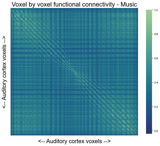
It is indeed a very large matrix… From this high-dimensional space, we will now obtain low-dimensional representations in manifold-space, i.e. gradients. To do so, we can utilize the Brainspace toolbox which comes with all the functions we need. It is as easy as setting up the GradientMaps class according to the parameters we want to use. Specifically, we want to extract 10 components, using diffusion map embedding ('dm'):
gm = GradientMaps(n_components=10, approach='dm', random_state=0)
Next, we need to fit it to our mean voxel by voxel functional connectivity matrix:
gm.fit(cor_music_mean)
GradientMaps(alignment=None, approach='dm', kernel=None, n_components=10,
random_state=0)
gm now contains the components and their respective eigenvalues. In order to decide which components to check further, we will evaluate the eigenvalues through a scree plot:
def plot_eigenvalues(gm, interactive=True):
var_exp = [(eig/sum(gm.lambdas_)*100) for eig in gm.lambdas_]
if interactive is False:
sns.set_context('paper')
sns.set_style('white')
plt.rcParams["font.family"] = "Arial"
f, ax = plt.subplots(figsize=(8, 8))
sns.scatterplot(range(gm.lambdas_.size), var_exp, ax=ax, s=90)
sns.lineplot(range(gm.lambdas_.size), var_exp, ax=ax)
plt.title('Variance explained per component - Music', fontsize=20)
plt.xticks(list(range(0,10)))
ax.set_xticklabels(list(range(1,11)))
ax.tick_params(axis='x', labelsize=15)
plt.xlabel('Component', fontsize=18)
plt.ylabel('Variance explained per component (%)', fontsize=18)
ax.tick_params(axis='y', labelsize=15)
sns.despine(offset=5)
else:
tmp_df = pd.DataFrame({'Component': range(gm.lambdas_.size), 'Variance explained': var_exp})
tmp_df['Component'] = tmp_df['Component']+1
fig = go.Figure(data=go.Scatter(x=tmp_df['Component'], y=tmp_df['Variance explained'],
mode='lines+markers',
marker=dict(size=16),
text=['Component %s' %str(int(comp+1)) for comp in tmp_df['Component']],
hovertemplate =
'<br><b>Component</b>: %{x}<br>'+
'<i>Variance explained</i>: %{y:.2f}'))
fig.update_layout(
autosize=False,
width=600,
height=600,)
fig['layout'].update(template='simple_white')
fig.update_layout(
title={
'text': "Variance explained per component - Music",
'y':0.90,
'x':0.5,
'xanchor': 'center',
'yanchor': 'top'},
xaxis_title="Component",
yaxis_title="Variance explained per component (%)",)
fig.update_xaxes(tickvals = list(range(1,11)))
plot(fig, filename = 'ac_network_cor-voxel_music.html')
display(HTML('ac_network_cor-voxel_music.html'))
plot_eigenvalues(gm)
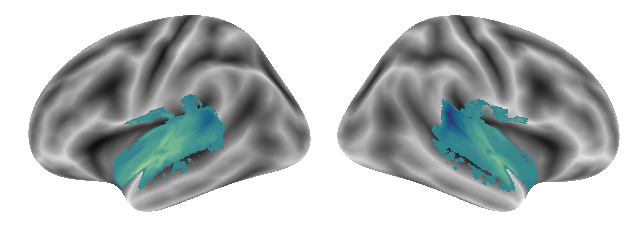
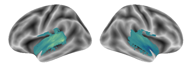
Based on these Eigenvalues/Variance explained and following prior research, we will focus on the first three components going further. First, we are of course interested in the spatial distribution, that is which voxels and thus regions behave alike across the beta series. To examine this, we need to transform the gradients back to brain images. This can be achieved by using the inverse transform of our NiftiMasker which will bring the gradients back to the auditory cortex. We will also create standardized versions of the gradients with values ranging between -1 and 1. A small for-loop will let us easily do that for the first three gradients:
list_grad_vols = []
scaler = MinMaxScaler(feature_range=(-1,1))
list_grad_vols_scaled = []
for grad in range(0,3):
list_grad_vols.append(ac_masker.inverse_transform(gm.gradients_.T[grad]))
list_grad_vols_scaled.append(ac_masker.inverse_transform(scaler.fit_transform(gm.gradients_.T[grad].reshape(-1,1)).reshape(-1)))
list_grad_vols now contains the first three gradients as images mapped back onto the auditory cortex. We can now plot them as any other brain image via setting up a comprehensive function:
def plot_gradients(gradient, surface=True, interactive=True, flipped=True, title=None):
fs_average = fetch_surf_fsaverage('fsaverage5')
if flipped is False:
grad_plot = gradient
else:
grad_plot = image.math_img("-img", img=gradient)
if title is None:
title = '[]'
else:
tile = title
if surface is False and interactive is False:
fig = plot_img(grad_plot, threshold=0.0001, bg_img=load_mni152_template(), cmap='crest_r', draw_cross=False, title=tile)
elif surface is True and interactive is False:
hemis= ['left', 'right']
modes = ['lateral']
aspect_ratio=1.4
surf = {
'left': fs_average['infl_left'],
'right': fs_average['infl_right'],
}
texture = {
'left': vol_to_surf(grad_plot, fs_average['pial_left']),
'right': vol_to_surf(grad_plot, fs_average['pial_right'])
}
figsize = plt.figaspect(len(modes) / (aspect_ratio * len(hemis)))
fig, axes = plt.subplots(nrows=len(modes),
ncols=len(hemis),
figsize=figsize,
subplot_kw={'projection': '3d'})
axes = np.atleast_2d(axes)
for index_mode, mode in enumerate(modes):
for index_hemi, hemi in enumerate(hemis):
bg_map = fs_average['sulc_%s' % hemi]
plot_surf_stat_map(surf[hemi], texture[hemi],
view=mode, hemi=hemi,
bg_map=bg_map,
axes=axes[index_mode, index_hemi],
colorbar=False,
threshold=0.0001,
cmap='crest_r', title=tile)
for ax in axes.flatten():
ax.dist = 6
fig.subplots_adjust(wspace=-0.02, hspace=0.0)
elif surface is False and interactive is True:
fig = view_img(grad_plot, cmap="crest_r", threshold=0.0001, black_bg=False, colorbar=True, draw_cross=False, bg_img=load_mni152_template(), title=tile)
elif surface is True and interactive is True:
fig = view_img_on_surf(grad_plot, cmap="crest_r", threshold=0.0001, black_bg=False, colorbar=True, surf_mesh=fs_average, title=tile)
return fig
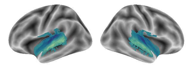
Let’s have a look at the first gradient:
plot_gradients(list_grad_vols_scaled[0], interactive=True, title='Gradient 1 - Music')
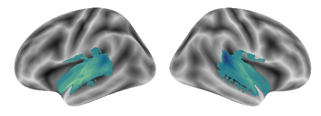
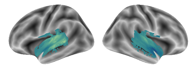
How does the second gradient look?
plot_gradients(list_grad_vols_scaled[1], interactive=True, title='Gradient 2 - Music')
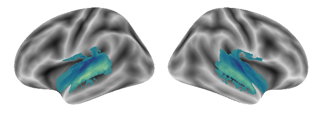
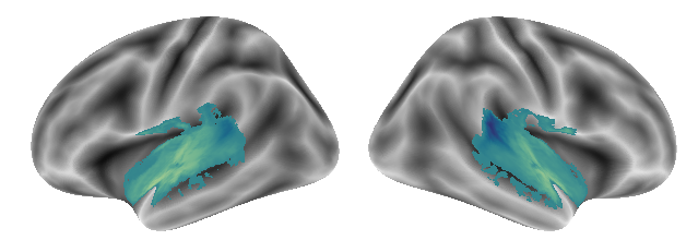
And what about the third gradient?
plot_gradients(list_grad_vols_scaled[2], interactive=True, title='Gradient 3 - Music')
Cool, we can definitely see some functional differentiations between voxels/regions that in parts resemble the proposed functional principles we are investigating. Let’s save the computed outputs that got us here: the beta series, the correlation matrix and both versions of the gradients, the original and scaled ones.
np.save(opj(results_path,'voxel_to_voxel/beta-series_%s_mask-ac.npy' %('Music')), bs_stack)
np.save(opj(results_path,'voxel_to_voxel/cor-mats_%s_ac_mask.npy' %('Music')), cor_music)
grad_vols = nb.concat_images(list_grad_vols)
grad_vols.to_filename(opj(results_path, 'voxel_to_voxel/group-level_gradient_task-%s.nii.gz' %('Music')))
grad_vols_scaled = nb.concat_images(list_grad_vols_scaled)
grad_vols_scaled.to_filename(opj(results_path, 'voxel_to_voxel/group-level_gradient_task-%s_desc-scaled.nii.gz' %('Music')))
Having all the functions we need to compute and assess voxel to voxel functional connectivity matrics and gradients, we can pack the different pieces into overarching functions to save space and time when investigating the other conditions. In more detail, we already have on for plotting and thus we will create one other function for computing and saving gradients and corresponding data:
def compute_gradients(condition, interactive=True):
ac_masker = NiftiMasker(mask_img=opj(roi_mask_path,'tpl-MNI152NLin6Sym_res_02_desc-AC_mask.nii.gz'),
standardize=True)
bs_tmp = []
for i, beta_series in enumerate(np.array(list_beta)[beta_series_info.condition.isin(condition)]):
bs_tmp.append(ac_masker.fit_transform(beta_series))
bs_stack = []
for i, part in enumerate(beta_series_info[beta_series_info.condition.isin(condition)]['participant'].unique()):
bs_stack.append(np.vstack(np.array(bs_tmp)[beta_series_info[beta_series_info.condition.isin(condition)].participant.isin([part])]))
cor_measure = ConnectivityMeasure(kind='correlation')
cor_tmp = cor_measure.fit_transform(bs_stack)
cor_tmp_mean = np.mean(cor_tmp, axis=0)
gm = GradientMaps(n_components=10, approach='dm', random_state=0)
gm.fit(cor_tmp_mean)
list_grad_vols = []
scaler = MinMaxScaler(feature_range=(-1,1))
list_grad_vols_scaled = []
for grad in range(0,3):
list_grad_vols.append(ac_masker.inverse_transform(gm.gradients_.T[grad]))
list_grad_vols_scaled.append(ac_masker.inverse_transform(scaler.fit_transform(gm.gradients_.T[grad].reshape(-1,1)).reshape(-1)))
grad_vols = nb.concat_images(list_grad_vols)
grad_vols_scaled = nb.concat_images(list_grad_vols_scaled)
if len(condition) == 1:
np.save(opj(results_path,'voxel_to_voxel/beta-series_%s_mask-ac.npy' %(condition[0])), bs_stack)
np.save(opj(results_path,'voxel_to_voxel/cor-mats_%s_ac_mask.npy' %condition[0]), cor_tmp)
grad_vols.to_filename(opj(results_path, 'voxel_to_voxel/group-level_gradient_task-%s.nii.gz' %condition[0]))
grad_vols_scaled.to_filename(opj(results_path, 'voxel_to_voxel/group-level_gradient_task-%s_desc-scaled.nii.gz' %condition[0]))
title_condition = condition[0]
elif len(condition) == 2:
np.save(opj(results_path,'voxel_to_voxel/beta-series_%s_mask-ac.npy' %(condition[0]+'-'+condition[1])), bs_stack)
np.save(opj(results_path,'voxel_to_voxel/cor-mats_%s_ac_mask.npy' %(condition[0]+'-'+condition[1])), cor_tmp)
grad_vols.to_filename(opj(results_path, 'voxel_to_voxel/group-level_gradient_task-%s.nii.gz' %(condition[0]+'-'+condition[1])))
grad_vols_scaled.to_filename(opj(results_path, 'voxel_to_voxel/group-level_gradient_task-%s_desc-scaled.nii.gz' %(condition[0]+'-'+condition[1])))
title_condition = (condition[0]+'-'+condition[1])
else:
np.save(opj(results_path,'voxel_to_voxel/beta-series_%s_mask-ac.npy' %(condition[0]+'-'+condition[1]+'-'+condition[2])), bs_stack)
np.save(opj(results_path,'voxel_to_voxel/cor-mats_%s_ac_mask.npy' %(condition[0]+'-'+condition[1]+'-'+condition[2])), cor_tmp)
grad_vols.to_filename(opj(results_path, 'voxel_to_voxel/group-level_gradient_task-%s.nii.gz' %(condition[0]+'-'+condition[1]+'-'+condition[2])))
grad_vols_scaled.to_filename(opj(results_path, 'voxel_to_voxel/group-level_gradient_task-%s_desc-scaled.nii.gz' %(condition[0]+'-'+condition[1]+'-'+condition[2])))
title_condition = (condition[0]+'-'+condition[1]+'-'+condition[2])
var_exp = [(eig/sum(gm.lambdas_)*100) for eig in gm.lambdas_]
if interactive is False:
sns.set_style('white')
plt.rcParams["font.family"] = "Arial"
fig, axes = plt.subplots(1,2, figsize = (20, 10))#, gridspec_kw={'width_ratios': [2, 2],
#'height_ratios': [1,1,1]})#, sharey=True)
sns.heatmap(cor_tmp_mean, cmap='crest_r', ax=axes[0], square=True, cbar_kws={'shrink':0.74})
axes[0].set_xlabel('<-- Auditory cortex voxels -->', fontsize=20)
axes[0].set_xticklabels([''])
axes[0].set_ylabel('<-- Auditory cortex voxels -->', fontsize=20)
axes[0].set_yticklabels([''])
axes[0].set_title('Voxel by voxel functional connectivity', fontsize=20)
pos1 = axes[0].get_position().bounds
sns.scatterplot(range(gm.lambdas_.size), var_exp, ax=axes[1], s=90)
sns.lineplot(range(gm.lambdas_.size), var_exp, ax=axes[1])
axes[1].set_title('Variance explained per component', fontsize=20)
axes[1].set_xticks(list(range(0,10)))
axes[1].set_xticklabels(list(range(1,11)))
axes[1].tick_params(axis='x', labelsize=15)
axes[1].set_xlabel('Component', fontsize=18)
axes[1].set_ylabel('Variance explained (%)', fontsize=18)
axes[1].tick_params(axis='y', labelsize=15)
sns.despine(offset=5,ax=axes[1])
axes[1].set_position([pos1[0]+0.48, pos1[1]+0.01, pos1[0]+0.15, pos1[1]+0.33])
fig.suptitle('Functional connectivity and gradients within the auditory cortex \n condition - %s' %title_condition, size=25)
plt.text(-4.7, 11, 'diffusion map\n embedding', fontsize=12)
plt.text(-4.2, 10.7, 'n=10', fontsize=12)
path = plt.arrow(-4.65, 10.9, 1.55, 0, ec="none", color='black', width=0.01, head_width=0.1, head_length=0.2, clip_on=False)
plt.show()
else:
fig = make_subplots(rows=2, cols=1,
subplot_titles=('Voxel by voxel functional connectivity', 'Variance explained per component'),
vertical_spacing=0.2)
fig.add_trace(go.Heatmap(z=cor_tmp_mean[:230,:230],
colorscale='darkmint_r', transpose=True, showscale=False), row=1, col=1)
tmp_df = pd.DataFrame({'Component': range(gm.lambdas_.size), 'Variance explained': var_exp})
tmp_df['Component'] = tmp_df['Component']+1
fig.add_trace(go.Scatter(x=tmp_df['Component'], y=tmp_df['Variance explained'],
mode='lines+markers',
marker=dict(size=16, color='steelblue'),
text=['Component %s' %str(int(comp+1)) for comp in tmp_df['Component']],
hovertemplate =
'<br><b>Component</b>: %{x}<br>'+
'<i>Variance explained</i>: %{y:.2f}'), row=2, col=1)
fig.update_layout(
autosize=False,
width=600,
height=1300,)
fig['layout'].update(template='simple_white')
fig.update_layout(
title={
'text': "Functional connectivity and gradients within the auditory cortex<br>condition - %s" %title_condition,
'y':0.99,
'x':0.5,
'xanchor': 'center',
'yanchor': 'top'})
fig['layout']['xaxis2']['tickvals'] = list(range(1,11))
fig['layout']['xaxis']['title']='<-- Auditory cortex voxels -->'
fig['layout']['xaxis2']['title']='Component'
fig['layout']['yaxis']['title']='<-- Auditory cortex voxels -->'
fig['layout']['yaxis2']['title']='Variance explained (%)'
fig['layout']['yaxis']['autorange'] = "reversed"
fig.add_annotation(text="diffusion map<br>embedding",
xref="paper", yref="paper",
x=0.40, y=0.49, showarrow=False)
fig.add_annotation(
xref="paper", yref="paper",
x=0.5, y=0.455, ax=0, ay=-80, showarrow=True,
arrowsize=1, arrowhead=3)
fig.add_annotation(text="n=10",
xref="paper", yref="paper",
x=0.55, y=0.49, showarrow=False)
plot(fig, filename = 'fc-gradients_%s.html' %title_condition)
display(HTML('fc-gradients_%s.html' %title_condition))
return list_grad_vols, list_grad_vols_scaled, gm
Again, a very long function. However, given all the things it is doing, the length and complexity is fair. Now we can easily compute and visualize voxel by voxel functional connectivity matrices and gradients for each condition and each combination of conditions. We will do this to inspect of certain conditions or combination of conditions results in different gradients.
Diffusion map embedding - Gradients - Voice
The first condition we will inspect is voice. Using our function from above, this is as easy as:
grad_vols_voice, grad_vols_voice_scaled, gm_voice = compute_gradients(['Voice'], interactive=True)
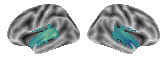
We can now inspect the gradients using our plotting function from above, starting with gradient 1:
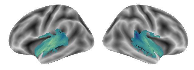
plot_gradients(grad_vols_voice_scaled[0], interactive=False)
followed by gradient 2:
plot_gradients(grad_vols_voice_scaled[1], interactive=False)
and finally gradient 3:
plot_gradients(grad_vols_voice_scaled[2], interactive=False)

Great, as said: easy and straightforward. We continue with Singing:
Diffusion map embedding - Gradients - Singing
grad_vols_singing, grad_vols_singing_scaled, gm_singing = compute_gradients(['Singing'], interactive=True)
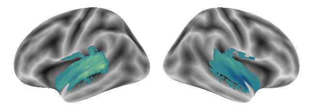
Let’s plot the gradients again, starting with 1:
plot_gradients(grad_vols_singing_scaled[0], interactive=False)
Here is gradient 2:
plot_gradients(grad_vols_singing_scaled[1], interactive=False)
And this is gradient 3:
plot_gradients(grad_vols_singing_scaled[2], interactive=False)
Now that we evaluated gradients for all conditions separately, we will check gradients based on condition pairs. Let’s start with voice and singing.
Diffusion map embedding - Gradients - Voice & Singing
Using our function, we can simply provide a list of two conditions instead of one to compute voxel by voxel functional connectivity and gradients based on a pair of conditions:
grad_vols_voice_singing, grad_vols_voice_singing_scaled, gm_voice_singing = compute_gradients(['Voice', 'Singing'], interactive=True)
So far, the outcomes look comparable to the single condition ones. What about the gradients? As before, we plot the gradients using our function, starting with gradient 1:
plot_gradients(grad_vols_voice_singing_scaled[0], interactive=False)

Here is gradient 2:
plot_gradients(grad_vols_voice_singing_scaled[1], interactive=False)
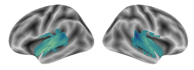
Gradient 3 for the voice and singing condition looks like the following:
plot_gradients(grad_vols_voice_singing_scaled[2], interactive=False)
Overall, we see no striking differences compared to the gradients before. Next up is the voice & music condition pair.
Diffusion map embedding - Gradients - Voice & Music
No surprise: the first step is our function to compute functional connectivity between voxels and gradients:
grad_vols_voice_music, grad_vols_voice_music_scaled, gm_voice_music = compute_gradients(['Voice', 'Music'], interactive=True)
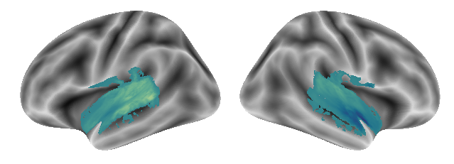
The following gradients were obtained from this condition pair, at first gradient 1:
plot_gradients(grad_vols_voice_music_scaled[0], interactive=False)

Gradient 2:
plot_gradients(grad_vols_voice_music_scaled[1], interactive=False)
and gradient 3:
plot_gradients(grad_vols_voice_music_scaled[2], interactive=False)
Again, no prominently different results. Let’s check the last condition pair: music and singing.
Diffusion map embedding - Gradients - Music & Singing
grad_vols_music_singing, grad_vols_music_singing_scaled, gm_music_singing = compute_gradients(['Music', 'Singing'], interactive=True)
The corresponding gradients from 1 to 3:
plot_gradients(grad_vols_music_singing_scaled[0], interactive=False)

plot_gradients(grad_vols_music_singing_scaled[1], interactive=False)
plot_gradients(grad_vols_music_singing_scaled[2], interactive=False)
After computing functional connectivity between voxels and gradients for each condition separately and each condition pair, we will do the same including all three conditions: voice, singing and music.
Diffusion map embedding - Gradients - Voice, Singing & Music
grad_vols_voice_singing_music, grad_vols_voice_singing_music_scaled, gm_voice_singing_music = compute_gradients(['Voice', 'Singing', 'Music'], interactive=True)
The first gradient we obtain from including all three conditions looks like this:
plot_gradients(grad_vols_voice_singing_music_scaled[0], interactive=False)

Here is the second gradient:
plot_gradients(grad_vols_voice_singing_music_scaled[1], interactive=False)

and here the third gradient:
plot_gradients(grad_vols_voice_singing_music_scaled[2], interactive=False)
This concludes this analyses step within which we derived variance explaining gradients in low-level manifold space from the voxel by voxel functional connectivity matrix. While we already produced a lot of graphics, we will investigate another one in the next step.
Diffusion map embedding - component plots
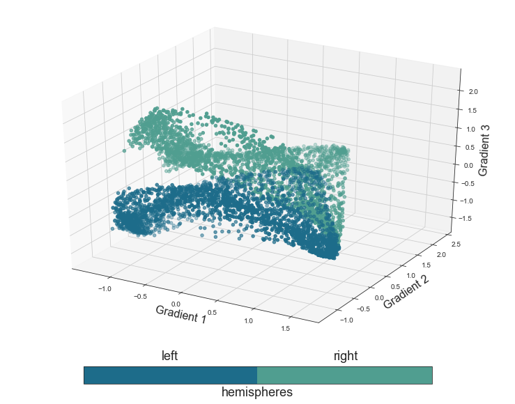
So far, we produced plots that show the voxel by voxel functional connectivity matrix, the components derived through diffusion map embedding and how much variance they explained, as well as the components transformed back to a 3D image to evaluate their spatial pattern. However, yet another interesting approach to plot the components in order to investigate if the reflect/indicate the proposed functional principles is to visualize the first three components via a 3D scatter plot within which we plot each component against one another. The result will be a 3D plot where each voxel is placed at a point in space based on its value in the first three components. The question concerning functional principles can be incorporate by coloring the voxels based on their location in the auditory cortex. To do this end, we will define a function that creates the 3D scatter plot and colors the voxels based on the auditory cortex ROI they belong to. We will include the functional principles as respective coloring mode. As usual within this resource, the function is quite long and complex, but through defining it like that once, we save a lot of time and space later on. Here is the function:
def plot_components_3d(mode=None, interactive=False, bg_white=False):
ac_masker = NiftiMasker(mask_img=opj(roi_mask_path,'tpl-MNI152NLin6Sym_res_02_desc-AC_mask.nii.gz'),standardize=True)
ac_atlas = opj(prereq_path, 'atlas/tpl-MNI152NLin2009cAsym_res-02_desc-ACatlas.nii.gz')
ac_mask_regions_values = ac_masker.fit_transform(ac_atlas)
if mode is None:
print('Please define a coloring mode.')
elif mode == 'hemi':
gradient_regions_hemi = []
for grad, reg in zip(gm_voice_singing_music.gradients_.T[1], ac_mask_regions_values.reshape(-1)):
if reg in [1,3,5,7,9]:
gradient_regions_hemi.append(1)
else:
gradient_regions_hemi.append(2)
colors = gradient_regions_hemi
cbar_label = 'hemispheres'
annot_left = 'left'
annot_right = 'right'
cmap = ListedColormap(sns.color_palette("crest_r", 2).as_hex())
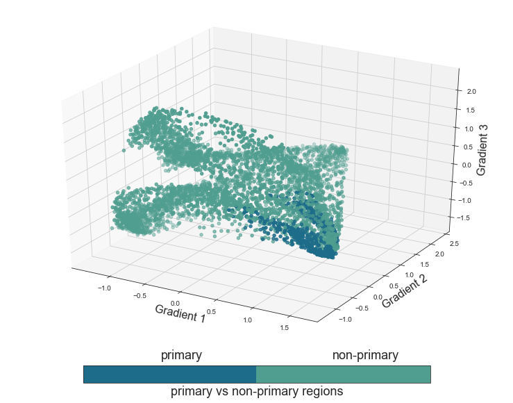
elif mode == 'primary':
gradient_regions_prim = []
for grad, reg in zip(gm_voice_singing_music.gradients_.T[1], ac_mask_regions_values.reshape(-1)):
if reg in [1,2]:
gradient_regions_prim.append(1)
else:
gradient_regions_prim.append(2)
colors = gradient_regions_prim
cbar_label = 'primary vs non-primary regions'
annot_left = 'primary'
annot_right = 'non-primary'
cmap = ListedColormap(sns.color_palette("crest_r", 2).as_hex())
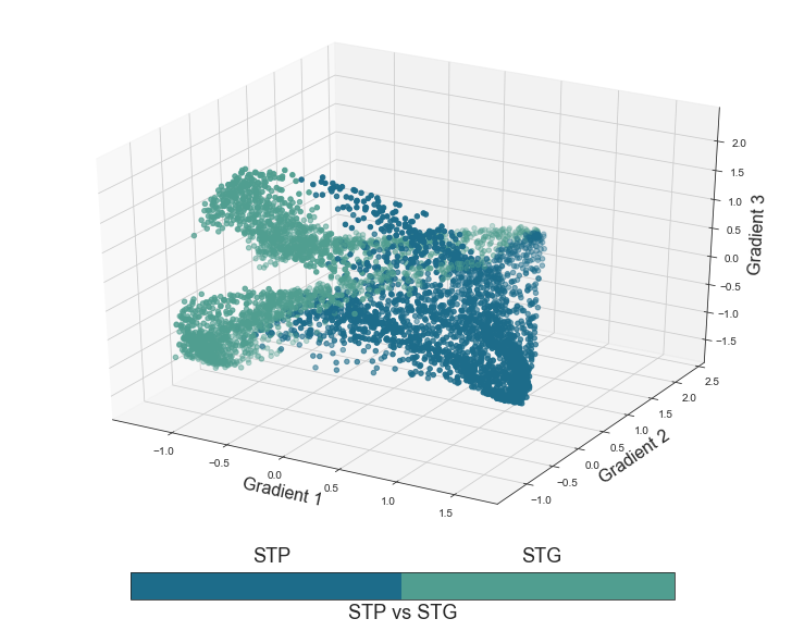
elif mode == 'stpstg':
gradient_regions_stpg = []
for grad, reg in zip(gm_voice_singing_music.gradients_.T[1], ac_mask_regions_values.reshape(-1)):
if reg in [1,2,3,4,5,6]:
gradient_regions_stpg.append(1)
else:
gradient_regions_stpg.append(2)
colors = gradient_regions_stpg
cbar_label = 'STP vs STG'
annot_left = 'STP'
annot_right = 'STG'
cmap = ListedColormap(sns.color_palette("crest_r", 2).as_hex())
elif mode == 'antpost':
gradient_regions_antpost = []
for grad, reg in zip(gm_voice_singing_music.gradients_.T[1], ac_mask_regions_values.reshape(-1)):
if reg in [5,6,9,10]:
gradient_regions_antpost.append(1)
elif reg in [1,2]:
gradient_regions_antpost.append(2)
else:
gradient_regions_antpost.append(3)
colors = gradient_regions_antpost
cbar_label = 'posterior vs anterior'
annot_left = 'posterior'
annot_center = 'primary'
annot_right = 'anterior'
cmap = ListedColormap(sns.color_palette("mako", 3).as_hex())
elif mode == 'roi':
gradient_regions_all = []
for grad, reg in zip(gm_voice_singing_music.gradients_.T[1], ac_mask_regions_values.reshape(-1)):
if reg == 10:
gradient_regions_all.append(1)
elif reg == 9:
gradient_regions_all.append(2)
elif reg == 6:
gradient_regions_all.append(3)
elif reg == 5:
gradient_regions_all.append(4)
elif reg == 2:
gradient_regions_all.append(5)
elif reg == 1:
gradient_regions_all.append(6)
elif reg == 4:
gradient_regions_all.append(7)
elif reg == 3:
gradient_regions_all.append(8)
elif reg == 8:
gradient_regions_all.append(9)
elif reg == 7:
gradient_regions_all.append(10)
colors = gradient_regions_all
cbar_label = 'posterior vs anterior per region & hemisphere'
annot_left = 'posterior'
annot_center = 'primary'
annot_right = 'anterior'
cmap = ListedColormap(sns.color_palette("mako", 10).as_hex())
if interactive is False:
sns.set_style('white')
plt.rcParams["font.family"] = "Arial"
fig = plt.figure(figsize=(13,10))
ax = plt.axes(projection="3d")
if bg_white is True:
ax.xaxis.set_pane_color((1.0, 1.0, 1.0, 0.0))
ax.yaxis.set_pane_color((1.0, 1.0, 1.0, 0.0))
ax.zaxis.set_pane_color((1.0, 1.0, 1.0, 0.0))
ax.xaxis._axinfo["grid"]['color'] = (1,1,1,0)
ax.yaxis._axinfo["grid"]['color'] = (1,1,1,0)
ax.zaxis._axinfo["grid"]['color'] = (1,1,1,0)
points = ax.scatter3D(gm_voice_singing_music.gradients_.T[0], gm_voice_singing_music.gradients_.T[1], gm_voice_singing_music.gradients_.T[2],
c=colors, cmap=cmap)
cbar=fig.colorbar(points, orientation='horizontal',
ticks=[], fraction=0.046, pad=0.06, aspect=20)
cbar.set_label(cbar_label, fontsize=18)
ax.set_xlabel('Gradient 1', fontsize=16)
ax.set_ylabel('Gradient 2', fontsize=16)
ax.set_zlabel('Gradient 3', fontsize=16)
if mode in ['hemi', 'primary', 'stpstg']:
ax.text2D(0.31, -0.05, annot_left, transform=ax.transAxes, fontsize=18)
ax.text2D(0.65, -0.05, annot_right, transform=ax.transAxes, fontsize=18)
else:
ax.text2D(0.23, -0.05, annot_left, transform=ax.transAxes, fontsize=18)
ax.text2D(0.46, -0.05, annot_center, transform=ax.transAxes, fontsize=18)
ax.text2D(0.69, -0.05, annot_right, transform=ax.transAxes, fontsize=18)
else:
import plotly.graph_objects as go
fig = go.Figure(data=[go.Scatter3d(x=gm_voice_singing_music.gradients_.T[0], y=gm_voice_singing_music.gradients_.T[1],
z=gm_voice_singing_music.gradients_.T[2],mode='markers', marker=dict(
size=12,
color=colors, # set color to an array/list of desired values
colorscale='darkmint_r', # choose a colorscale
opacity=0.6
))])
fig.update_layout(
autosize=False,
width=1300,
height=600,)
fig['layout'].update(template='simple_white')
fig.show()
Great, now we can generate the plots. Please note that we will do this only for the last gradients we assessed, the one including all three conditions, as this was the one we focused on in the publication as well. We will start with the functional principle hemispheres, that is color the voxels based on the hemisphere they belong to.
plot_components_3d(mode='hemi', interactive=False)
Nice to see our function working as expected. Let’s continue with the next functional principle, the proposed distinction between primary and non-primary regions:
plot_components_3d(mode='primary', interactive=False)
Coming up next, is the STP vs. STG functional principle, assuming a differentiation between voxels in the STP and those in the STG.
plot_components_3d(mode='stpstg', interactive=False)
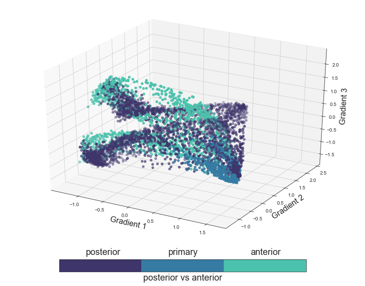
The next functional principle we will evaluate is the distinction between anterior and posterior regions. Given that we can not include the primary regions in either, we will color the voxels based on primary, anterior and posterior regions.
plot_components_3d(mode='antpost', interactive=False)
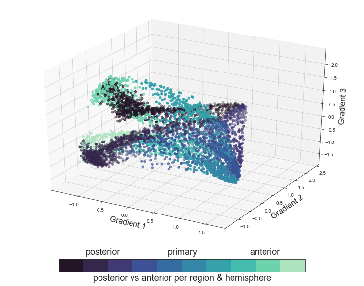
Having created graphics based on all proposed functional principles, we all generate a final plot within which we will color the voxels based on the auditory cortex ROI they belong to and not group them in order to obtain even more detailed insights.
plot_components_3d(mode='roi', interactive=False)
This was the final step of both the voxel to voxel correlation and the connectivity analyses as a whole. Throughout this section we investigated if the task based functional connectivity induced through our conditions reflects/indicates aspects of the functional principles on two spatial scales: between ROIs and between voxels.
Summary and outlook
Next up, meta-analyses!