Build and train your neural network¶

Aim(s) for this section 🎯¶

get practical experience with ANNs, specifically CNNs
built, train and evalaute a CNN
discuss important building blocks and learn how to interpret outcomes

Outline for this section 📝¶

The tutorial dataset
- preparing the data
Building and training an ANN - a 2D CNN example
- python and deep learning
- defining the basics
- building an ANN
- how to train your network
Evaluating an ANN
- The test set
- Confusion matrix
- Generalization
- Transfer learning

import random
random.seed(0)

The tutorial dataset¶

In order to demonstrate how you can build and train an ANN we need a dataset that fits several requirements:

we are all here with laptops that most likely don’t have the computational power of HPCs and graphic cards (if you do, good for you!), thus the dataset needs to be small enough so that we can actually train our ANN within a short amount of time and without GPUs
thinking this further: we also might not want to test the most simplest ANN, but one with a few hidden layers
it would be cool to use a dataset with at least some real world feeling to demonstrate a somewhat typical workflow

We thus decided on a small fMRI dataset from Zhang et al. with the following specs:

two resting-state sessions from 48 participants
one with eyes-closed and one with eyes-open
we will use a subset of volumes of each session

This will allow us to:

address a (somewhat) realistic image processing task via supervised learning for which we can employ a CNN
showcase how parameters might change the ANN
evaluate representations across layers

A note on the datasets utilized here:

we’re very sorry that it’s so (f)MRI focused
we tried to include other modalities, specifically microscopy, but:
- couldn’t find datasets that fit the setup and framework of the workshop
- don’t have enough experience with this modality to adapt existing ones
however, we collected a few resources on machine and deep learning for microscopy here
- contain a variety of pre-trained models
- info on how to prepare data
we also tested and checked a few things in advance so that we can help you during the hands-on in the best way possible

_{^{_{^{^{https://media4.giphy.com/media/rvDtLCABDMaqY/giphy.gif?cid=ecf05e47c5qyer72l87resjeadw2zu6kdoqq1b6guo8gqr9d&rid=giphy.gif&ct=g}}}}}

that being said, let’s gather our dataset

import urllib.request

url = 'https://github.com/miykael/workshop_pybrain/raw/master/workshop/notebooks/data/dataset_ML.nii.gz'
urllib.request.urlretrieve(url, 'dataest_ML.nii.gz')

('dataest_ML.nii.gz', <http.client.HTTPMessage at 0x7fe3a7f6f370>)

and check its dimensions as well as visually inspect it:

import nibabel as nb

data = nb.load('dataest_ML.nii.gz')

data.shape

(40, 51, 41, 384)

data.orthoview()

<OrthoSlicer3D: dataest_ML.nii.gz (40, 51, 41, 384)>

../../../_images/DL_build_train_15_1.png

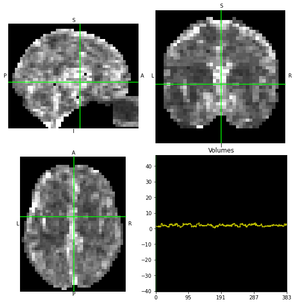
We can also plot the mean image across time to get an idea about signal variation:

from nilearn.image import mean_img
from nilearn.plotting import view_img

/Users/peerherholz/anaconda3/envs/ml-dl-synage/lib/python3.8/site-packages/nilearn/datasets/__init__.py:86: FutureWarning: Fetchers from the nilearn.datasets module will be updated in version 0.9 to return python strings instead of bytes and Pandas dataframes instead of Numpy arrays.
  warn("Fetchers from the nilearn.datasets module will be "

view_img(mean_img(data))

Well well well, there should be something in there that an ANN can learn…

the task:
- we know that there are images where participants had their eyes open or closed
- we now want to build an ANN to train it to recognize and distinguish the respective images
- we also want to know what representations our ANN learns
- thus, we have a supervised learning problem which we want to solve via image processing

what we need to do:
- prepare the data
- decide on a model, build and train it

Preparing the data

From our adventures in "classic" machine learning we know, that we need labels to address a supervised learning problem. Checking the dimensions of our dataset again:

data.shape

(40, 51, 41, 384)

We see that we have a 4 dimensional dataset, with the first three dimensions being spatial, i.e. x, y and z, and the fourth being time. So we need to specify during which of the images participants had their eyes closed and during which they had their eyes open. Without going into further detail, we know that it’s always 4 volumes of eyes closed, followed by 4 volumes of eyes open, etc. and given that we have 48 participants, we can define our labels as follows:

import numpy as np

labels = np.ravel([[['closed'] * 4, ['open'] * 4] for i in range(48)])
labels[:20]

array(['closed', 'closed', 'closed', 'closed', 'open', 'open', 'open',
       'open', 'closed', 'closed', 'closed', 'closed', 'open', 'open',
       'open', 'open', 'closed', 'closed', 'closed', 'closed'],
      dtype='<U6')

Going back to the aspect of computation time and resources, as well as given that this is a showcase, it might be a good idea to not utilize the entire fMRI volume, but only certain parts where we expect some things to happen. (Please note: this is of course a form of inductive bias comparable to feature engineering in "classic" machine learning and something you won’t do in a “real-world situation” (depending on the data and goal of course)).

In our case, we could try to not train the neural network only on one very thin slab (a few slices) of the brain. So, instead of taking the data matrix of the whole brain, we just take 2 slices in the region that we think is most likely to be predictive for the question at hand.

We know (or suspect) that the regions with the most predictive power are probably somewhere around the eyes and in the visual cortex. So let’s try to specify a few slices that cover those regions.

So, let’s try to just take a few slices around the eyes:

from nilearn.plotting import plot_img
plot_img(mean_img(data).slicer[...,5:-25], cmap='magma', colorbar=False,
          display_mode='x', vmax=2, annotate=False, cut_coords=range(0, 49, 12),
          title='Slab of the mean image');

../../../_images/DL_build_train_29_0.png

This worked only so and so, but with a few lines of code the mighty power of python and its packages can help us achieve a better training dataset. For example, we could rotate the volume (depending on the data and goal, this sort of image processing is actually sometimes done in “real-world situations”):

# Rotation parameters
phi = 0.35
cos = np.cos(phi)
sin = np.sin(phi)

# Compute rotation matrix around x-axis
rotation_affine = np.array([[1, 0, 0, 0],
                            [0, cos, -sin, 0],
                            [0, sin, cos, 0],
                            [0, 0, 0, 1]])
new_affine = rotation_affine.dot(data.affine)

Now we can use this new affine to resample our volumes:

from nilearn.image import resample_img
new_img = nb.Nifti1Image(data.get_fdata(), new_affine)
img_rot = resample_img(new_img, data.affine, interpolation='continuous')

How do our volumes look now?

plot_img(mean_img(img_rot).slicer[...,5:-25], cmap='magma', colorbar=False,
          display_mode='x', vmax=2, annotate=False, cut_coords=range(0, 49, 12),
          title='Slab of the mean rotated image');

../../../_images/DL_build_train_35_0.png

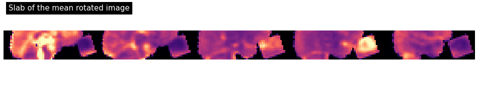
Coolio! Now we can check what set of slices of our volumes might constitute feasible inputs to our ANN:

from nilearn.plotting import plot_stat_map
img_slab = img_rot.slicer[..., 12:15, :]
plot_stat_map(mean_img(img_slab), cmap='magma', bg_img=mean_img(img_slab), colorbar=False,
              display_mode='x', vmax=2, annotate=False, cut_coords=range(-20, 30, 12),
              title='Slices of the rotated image');

../../../_images/DL_build_train_37_0.png

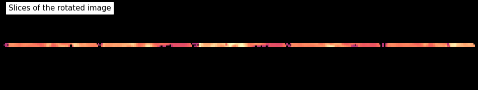
Now this is something we can definitely work with, even if we have only limited time and resources.

Building and training an `ANN` - a `2D CNN` example¶

Not that we have checked and further prepared our dataset, it’s finally time to get to work. Given that we’re working with fMRI volumes, i.e. images and what we’ve heard about the different ANN architectures, using a CNN might be a good idea.

But where to start? Is there any software I can use that makes the building, training and evaluating of ANNs “comparably easy”?

Well, say no more…Python obviously also has your back when it’s about deep learning (gotta love python, eh?)! It actually has not only but a bunch of different packages that focus on deep learning. Let’s have a brief look on the things that are out there.

Python and `deep learning`¶

As outlined before python is a very powerful all purpose language, including a broad user base and support for machine learning, both “classic” and deep learning.

logo _{^{_{^{https://miro.medium.com/max/1400/1*RIrPOCyMFwFC-XULbja3rw.png}}}}

lots of well documented and tested libraries
lots of tutorials to learn things (you + the ANN):
- youtube videos
- blog posts
- other open workshops
- jupyter notebooks
lots of pre-trained models to use for your research
lots of support in forums
completely free and open source!

_{^{_{^{https://miro.medium.com/max/700/1*s_BwkYxpGv34vjOHi8tDzg.png}}}}

all work a bit different, but the basic concepts and steps are comparable
- nevertheless: always check the documentation as e.g. default values might vary
crucial in all: tensors
- have a look at this great introduction to tensors from tensorflow

the question which one to choose is of course not an easy one and might also depend on external factors:
- the type and amount of data you have
- the time and computational resources available to you
- specific functionality that only exists in a certain package
- utilization of pre-trained ANNs
- what you’ve heard about and others show you (that’s obviously on us…)

here we will use keras which is build on top of tensorflow because:
- high-level API
- easy to grasp implementation of ANN building blocks
- fast experimentation
for a fantastic resource that includes all things we talked about/will talk and way more in much greater detail, please check the deep learning part of Neuromatch Academy

important: we’re not saying that keras/tensorflow is better than the other python deep learning libraries, it just works very well for tutorials/workshops like the one you’re currently at given the very limited time we have

Now it’s finally go time, get your machines ready!

_{^{_{^{^{https://c.tenor.com/1cbzhT0TKTMAAAAd/cat-asleep.gif}}}}}

Defining the basics¶

Before we can actually assemble our ANN, we need to set a few things. However, first things first: importing modules and classes:

from tensorflow.python.keras.models import Sequential
from tensorflow.python.keras.layers import Conv2D, MaxPooling2D, AvgPool2D, BatchNormalization
from tensorflow.python.keras.layers import Activation, Dropout, Flatten, Dense
from tensorflow.keras.optimizers import Adam

Next, we need to take a look at our dataset again, specifically its dimensions:

img_slab.shape

(40, 56, 3, 384)

Again, we have the x, y and z of our images, i.e. the images themselves, in the first three dimensions which are stacked in the fourth dimension. For this type of data to work with keras/tensorflow we actually need to adapt, that is swap, some of the dimensions, as these modules/functions expect them in a different way. This part of getting your data ready as input into a given ANN is crucial and can cause one or the other problem. Therefore, always make sure to carefully read the documentation of a class, module or pre-trained model you want to use. They are usually very good and show entail examples of how to get data ready for the ANN.

That being said, here we need basically only need to make the last dimension the first, so that we have the volumes/images stacked in the first dimension and the images themselves within the subsequent three:

data = np.rollaxis(img_slab.get_fdata(), 3, 0)
data.shape

(384, 40, 56, 3)

Specifically, the last dimension, here 3, are considered as channels.

There are some central parameters we can set before building the ANN itself. For example, we know the shape of the input. That is, the dimensions our input layer will receive:

data_shape = tuple(data.shape[1:])
data_shape

(40, 56, 3)

We also want to set the kernel size of our convolutional kernel. As heard before, this can be a tremendously important hyperparamter that can drastically affect the behavior of your ANN. It is thus something you have to carefully think about and even might want to evaluate via cross-validation. Here, we will use a kernel size of (3,3).

kernel_size = (3, 3)

The same holds true for the filters we want our convolutional layers to use:

filters = 32

Given that we want to work with a supervised learning problem and know that there are 2 classes we want our ANN to learn to learn distinguish, we can set the number of classes accordingly:

n_classes = 2

With that, we ready to start building our ANN!

Building an `ANN`¶

You heard right, it’s finally ANN time! Initially, we have to decide on an architecture, that is the type of ANN we want to build. As we want to test a simple CNN, a feedforward ANN without multiple inputs and/or outputs, we will employ what is called a sequential model in keras/tensorflows within which we define layer by layer. Note: It’s the easiest but also the most restrictive one.

model = Sequential()

2021-09-21 15:41:37.064283: I tensorflow/core/platform/cpu_feature_guard.cc:142] This TensorFlow binary is optimized with oneAPI Deep Neural Network Library (oneDNN) to use the following CPU instructions in performance-critical operations:  AVX2 FMA
To enable them in other operations, rebuild TensorFlow with the appropriate compiler flags.

Now that the basic structure is defined, we can start adding layers to our ANN. This is achieved by the following syntax (pseudocode):

model.add(layer_typ(layer_settings, layer_parameters))

Defining the `input layer`¶

The first step? Obviously defining an input layer, i.e. the layer that receives the external input. We want to build a CNN, so let’s make it a convolutional layer. What do we need for that?

help(Conv2D)

Help on class Conv2D in module tensorflow.python.keras.layers.convolutional:

class Conv2D(Conv)
 |  Conv2D(*args, **kwargs)
 |  
 |  2D convolution layer (e.g. spatial convolution over images).
 |  
 |  This layer creates a convolution kernel that is convolved
 |  with the layer input to produce a tensor of
 |  outputs. If `use_bias` is True,
 |  a bias vector is created and added to the outputs. Finally, if
 |  `activation` is not `None`, it is applied to the outputs as well.
 |  
 |  When using this layer as the first layer in a model,
 |  provide the keyword argument `input_shape`
 |  (tuple of integers or `None`, does not include the sample axis),
 |  e.g. `input_shape=(128, 128, 3)` for 128x128 RGB pictures
 |  in `data_format="channels_last"`. You can use `None` when
 |  a dimension has variable size.
 |  
 |  Examples:
 |  
 |  >>> # The inputs are 28x28 RGB images with `channels_last` and the batch
 |  >>> # size is 4.
 |  >>> input_shape = (4, 28, 28, 3)
 |  >>> x = tf.random.normal(input_shape)
 |  >>> y = tf.keras.layers.Conv2D(
 |  ... 2, 3, activation='relu', input_shape=input_shape[1:])(x)
 |  >>> print(y.shape)
 |  (4, 26, 26, 2)
 |  
 |  >>> # With `dilation_rate` as 2.
 |  >>> input_shape = (4, 28, 28, 3)
 |  >>> x = tf.random.normal(input_shape)
 |  >>> y = tf.keras.layers.Conv2D(
 |  ... 2, 3, activation='relu', dilation_rate=2, input_shape=input_shape[1:])(x)
 |  >>> print(y.shape)
 |  (4, 24, 24, 2)
 |  
 |  >>> # With `padding` as "same".
 |  >>> input_shape = (4, 28, 28, 3)
 |  >>> x = tf.random.normal(input_shape)
 |  >>> y = tf.keras.layers.Conv2D(
 |  ... 2, 3, activation='relu', padding="same", input_shape=input_shape[1:])(x)
 |  >>> print(y.shape)
 |  (4, 28, 28, 2)
 |  
 |  >>> # With extended batch shape [4, 7]:
 |  >>> input_shape = (4, 7, 28, 28, 3)
 |  >>> x = tf.random.normal(input_shape)
 |  >>> y = tf.keras.layers.Conv2D(
 |  ... 2, 3, activation='relu', input_shape=input_shape[2:])(x)
 |  >>> print(y.shape)
 |  (4, 7, 26, 26, 2)
 |  
 |  
 |  Args:
 |    filters: Integer, the dimensionality of the output space (i.e. the number of
 |      output filters in the convolution).
 |    kernel_size: An integer or tuple/list of 2 integers, specifying the height
 |      and width of the 2D convolution window. Can be a single integer to specify
 |      the same value for all spatial dimensions.
 |    strides: An integer or tuple/list of 2 integers, specifying the strides of
 |      the convolution along the height and width. Can be a single integer to
 |      specify the same value for all spatial dimensions. Specifying any stride
 |      value != 1 is incompatible with specifying any `dilation_rate` value != 1.
 |    padding: one of `"valid"` or `"same"` (case-insensitive).
 |      `"valid"` means no padding. `"same"` results in padding with zeros evenly
 |      to the left/right or up/down of the input such that output has the same
 |      height/width dimension as the input.
 |    data_format: A string, one of `channels_last` (default) or `channels_first`.
 |      The ordering of the dimensions in the inputs. `channels_last` corresponds
 |      to inputs with shape `(batch_size, height, width, channels)` while
 |      `channels_first` corresponds to inputs with shape `(batch_size, channels,
 |      height, width)`. It defaults to the `image_data_format` value found in
 |      your Keras config file at `~/.keras/keras.json`. If you never set it, then
 |      it will be `channels_last`.
 |    dilation_rate: an integer or tuple/list of 2 integers, specifying the
 |      dilation rate to use for dilated convolution. Can be a single integer to
 |      specify the same value for all spatial dimensions. Currently, specifying
 |      any `dilation_rate` value != 1 is incompatible with specifying any stride
 |      value != 1.
 |    groups: A positive integer specifying the number of groups in which the
 |      input is split along the channel axis. Each group is convolved separately
 |      with `filters / groups` filters. The output is the concatenation of all
 |      the `groups` results along the channel axis. Input channels and `filters`
 |      must both be divisible by `groups`.
 |    activation: Activation function to use. If you don't specify anything, no
 |      activation is applied (see `keras.activations`).
 |    use_bias: Boolean, whether the layer uses a bias vector.
 |    kernel_initializer: Initializer for the `kernel` weights matrix (see
 |      `keras.initializers`). Defaults to 'glorot_uniform'.
 |    bias_initializer: Initializer for the bias vector (see
 |      `keras.initializers`). Defaults to 'zeros'.
 |    kernel_regularizer: Regularizer function applied to the `kernel` weights
 |      matrix (see `keras.regularizers`). 
 |    bias_regularizer: Regularizer function applied to the bias vector (see
 |      `keras.regularizers`). 
 |    activity_regularizer: Regularizer function applied to the output of the
 |      layer (its "activation") (see `keras.regularizers`).
 |    kernel_constraint: Constraint function applied to the kernel matrix (see
 |      `keras.constraints`).
 |    bias_constraint: Constraint function applied to the bias vector (see
 |      `keras.constraints`).
 |  Input shape:
 |    4+D tensor with shape: `batch_shape + (channels, rows, cols)` if
 |      `data_format='channels_first'`
 |    or 4+D tensor with shape: `batch_shape + (rows, cols, channels)` if
 |      `data_format='channels_last'`.
 |  Output shape:
 |    4+D tensor with shape: `batch_shape + (filters, new_rows, new_cols)` if
 |    `data_format='channels_first'` or 4+D tensor with shape: `batch_shape +
 |      (new_rows, new_cols, filters)` if `data_format='channels_last'`.  `rows`
 |      and `cols` values might have changed due to padding.
 |  
 |  Returns:
 |    A tensor of rank 4+ representing
 |    `activation(conv2d(inputs, kernel) + bias)`.
 |  
 |  Raises:
 |    ValueError: if `padding` is `"causal"`.
 |    ValueError: when both `strides > 1` and `dilation_rate > 1`.
 |  
 |  Method resolution order:
 |      Conv2D
 |      Conv
 |      tensorflow.python.keras.engine.base_layer.Layer
 |      tensorflow.python.module.module.Module
 |      tensorflow.python.training.tracking.tracking.AutoTrackable
 |      tensorflow.python.training.tracking.base.Trackable
 |      tensorflow.python.keras.utils.version_utils.LayerVersionSelector
 |      builtins.object
 |  
 |  Methods defined here:
 |  
 |  __init__(self, filters, kernel_size, strides=(1, 1), padding='valid', data_format=None, dilation_rate=(1, 1), groups=1, activation=None, use_bias=True, kernel_initializer='glorot_uniform', bias_initializer='zeros', kernel_regularizer=None, bias_regularizer=None, activity_regularizer=None, kernel_constraint=None, bias_constraint=None, **kwargs)
 |  
 |  ----------------------------------------------------------------------
 |  Methods inherited from Conv:
 |  
 |  build(self, input_shape)
 |      Creates the variables of the layer (optional, for subclass implementers).
 |      
 |      This is a method that implementers of subclasses of `Layer` or `Model`
 |      can override if they need a state-creation step in-between
 |      layer instantiation and layer call.
 |      
 |      This is typically used to create the weights of `Layer` subclasses.
 |      
 |      Args:
 |        input_shape: Instance of `TensorShape`, or list of instances of
 |          `TensorShape` if the layer expects a list of inputs
 |          (one instance per input).
 |  
 |  call(self, inputs)
 |      This is where the layer's logic lives.
 |      
 |      Note here that `call()` method in `tf.keras` is little bit different
 |      from `keras` API. In `keras` API, you can pass support masking for
 |      layers as additional arguments. Whereas `tf.keras` has `compute_mask()`
 |      method to support masking.
 |      
 |      Args:
 |        inputs: Input tensor, or dict/list/tuple of input tensors.
 |          The first positional `inputs` argument is subject to special rules:
 |          - `inputs` must be explicitly passed. A layer cannot have zero
 |            arguments, and `inputs` cannot be provided via the default value
 |            of a keyword argument.
 |          - NumPy array or Python scalar values in `inputs` get cast as tensors.
 |          - Keras mask metadata is only collected from `inputs`.
 |          - Layers are built (`build(input_shape)` method)
 |            using shape info from `inputs` only.
 |          - `input_spec` compatibility is only checked against `inputs`.
 |          - Mixed precision input casting is only applied to `inputs`.
 |            If a layer has tensor arguments in `*args` or `**kwargs`, their
 |            casting behavior in mixed precision should be handled manually.
 |          - The SavedModel input specification is generated using `inputs` only.
 |          - Integration with various ecosystem packages like TFMOT, TFLite,
 |            TF.js, etc is only supported for `inputs` and not for tensors in
 |            positional and keyword arguments.
 |        *args: Additional positional arguments. May contain tensors, although
 |          this is not recommended, for the reasons above.
 |        **kwargs: Additional keyword arguments. May contain tensors, although
 |          this is not recommended, for the reasons above.
 |          The following optional keyword arguments are reserved:
 |          - `training`: Boolean scalar tensor of Python boolean indicating
 |            whether the `call` is meant for training or inference.
 |          - `mask`: Boolean input mask. If the layer's `call()` method takes a
 |            `mask` argument, its default value will be set to the mask generated
 |            for `inputs` by the previous layer (if `input` did come from a layer
 |            that generated a corresponding mask, i.e. if it came from a Keras
 |            layer with masking support).
 |      
 |      Returns:
 |        A tensor or list/tuple of tensors.
 |  
 |  compute_output_shape(self, input_shape)
 |      Computes the output shape of the layer.
 |      
 |      If the layer has not been built, this method will call `build` on the
 |      layer. This assumes that the layer will later be used with inputs that
 |      match the input shape provided here.
 |      
 |      Args:
 |          input_shape: Shape tuple (tuple of integers)
 |              or list of shape tuples (one per output tensor of the layer).
 |              Shape tuples can include None for free dimensions,
 |              instead of an integer.
 |      
 |      Returns:
 |          An input shape tuple.
 |  
 |  get_config(self)
 |      Returns the config of the layer.
 |      
 |      A layer config is a Python dictionary (serializable)
 |      containing the configuration of a layer.
 |      The same layer can be reinstantiated later
 |      (without its trained weights) from this configuration.
 |      
 |      The config of a layer does not include connectivity
 |      information, nor the layer class name. These are handled
 |      by `Network` (one layer of abstraction above).
 |      
 |      Note that `get_config()` does not guarantee to return a fresh copy of dict
 |      every time it is called. The callers should make a copy of the returned dict
 |      if they want to modify it.
 |      
 |      Returns:
 |          Python dictionary.
 |  
 |  ----------------------------------------------------------------------
 |  Methods inherited from tensorflow.python.keras.engine.base_layer.Layer:
 |  
 |  __call__(self, *args, **kwargs)
 |      Wraps `call`, applying pre- and post-processing steps.
 |      
 |      Args:
 |        *args: Positional arguments to be passed to `self.call`.
 |        **kwargs: Keyword arguments to be passed to `self.call`.
 |      
 |      Returns:
 |        Output tensor(s).
 |      
 |      Note:
 |        - The following optional keyword arguments are reserved for specific uses:
 |          * `training`: Boolean scalar tensor of Python boolean indicating
 |            whether the `call` is meant for training or inference.
 |          * `mask`: Boolean input mask.
 |        - If the layer's `call` method takes a `mask` argument (as some Keras
 |          layers do), its default value will be set to the mask generated
 |          for `inputs` by the previous layer (if `input` did come from
 |          a layer that generated a corresponding mask, i.e. if it came from
 |          a Keras layer with masking support.
 |        - If the layer is not built, the method will call `build`.
 |      
 |      Raises:
 |        ValueError: if the layer's `call` method returns None (an invalid value).
 |        RuntimeError: if `super().__init__()` was not called in the constructor.
 |  
 |  __delattr__(self, name)
 |      Implement delattr(self, name).
 |  
 |  __getstate__(self)
 |  
 |  __setattr__(self, name, value)
 |      Support self.foo = trackable syntax.
 |  
 |  __setstate__(self, state)
 |  
 |  add_loss(self, losses, **kwargs)
 |      Add loss tensor(s), potentially dependent on layer inputs.
 |      
 |      Some losses (for instance, activity regularization losses) may be dependent
 |      on the inputs passed when calling a layer. Hence, when reusing the same
 |      layer on different inputs `a` and `b`, some entries in `layer.losses` may
 |      be dependent on `a` and some on `b`. This method automatically keeps track
 |      of dependencies.
 |      
 |      This method can be used inside a subclassed layer or model's `call`
 |      function, in which case `losses` should be a Tensor or list of Tensors.
 |      
 |      Example:
 |      
 |      ```python
 |      class MyLayer(tf.keras.layers.Layer):
 |        def call(self, inputs):
 |          self.add_loss(tf.abs(tf.reduce_mean(inputs)))
 |          return inputs
 |      ```
 |      
 |      This method can also be called directly on a Functional Model during
 |      construction. In this case, any loss Tensors passed to this Model must
 |      be symbolic and be able to be traced back to the model's `Input`s. These
 |      losses become part of the model's topology and are tracked in `get_config`.
 |      
 |      Example:
 |      
 |      ```python
 |      inputs = tf.keras.Input(shape=(10,))
 |      x = tf.keras.layers.Dense(10)(inputs)
 |      outputs = tf.keras.layers.Dense(1)(x)
 |      model = tf.keras.Model(inputs, outputs)
 |      # Activity regularization.
 |      model.add_loss(tf.abs(tf.reduce_mean(x)))
 |      ```
 |      
 |      If this is not the case for your loss (if, for example, your loss references
 |      a `Variable` of one of the model's layers), you can wrap your loss in a
 |      zero-argument lambda. These losses are not tracked as part of the model's
 |      topology since they can't be serialized.
 |      
 |      Example:
 |      
 |      ```python
 |      inputs = tf.keras.Input(shape=(10,))
 |      d = tf.keras.layers.Dense(10)
 |      x = d(inputs)
 |      outputs = tf.keras.layers.Dense(1)(x)
 |      model = tf.keras.Model(inputs, outputs)
 |      # Weight regularization.
 |      model.add_loss(lambda: tf.reduce_mean(d.kernel))
 |      ```
 |      
 |      Args:
 |        losses: Loss tensor, or list/tuple of tensors. Rather than tensors, losses
 |          may also be zero-argument callables which create a loss tensor.
 |        **kwargs: Additional keyword arguments for backward compatibility.
 |          Accepted values:
 |            inputs - Deprecated, will be automatically inferred.
 |  
 |  add_metric(self, value, name=None, **kwargs)
 |      Adds metric tensor to the layer.
 |      
 |      This method can be used inside the `call()` method of a subclassed layer
 |      or model.
 |      
 |      ```python
 |      class MyMetricLayer(tf.keras.layers.Layer):
 |        def __init__(self):
 |          super(MyMetricLayer, self).__init__(name='my_metric_layer')
 |          self.mean = tf.keras.metrics.Mean(name='metric_1')
 |      
 |        def call(self, inputs):
 |          self.add_metric(self.mean(inputs))
 |          self.add_metric(tf.reduce_sum(inputs), name='metric_2')
 |          return inputs
 |      ```
 |      
 |      This method can also be called directly on a Functional Model during
 |      construction. In this case, any tensor passed to this Model must
 |      be symbolic and be able to be traced back to the model's `Input`s. These
 |      metrics become part of the model's topology and are tracked when you
 |      save the model via `save()`.
 |      
 |      ```python
 |      inputs = tf.keras.Input(shape=(10,))
 |      x = tf.keras.layers.Dense(10)(inputs)
 |      outputs = tf.keras.layers.Dense(1)(x)
 |      model = tf.keras.Model(inputs, outputs)
 |      model.add_metric(math_ops.reduce_sum(x), name='metric_1')
 |      ```
 |      
 |      Note: Calling `add_metric()` with the result of a metric object on a
 |      Functional Model, as shown in the example below, is not supported. This is
 |      because we cannot trace the metric result tensor back to the model's inputs.
 |      
 |      ```python
 |      inputs = tf.keras.Input(shape=(10,))
 |      x = tf.keras.layers.Dense(10)(inputs)
 |      outputs = tf.keras.layers.Dense(1)(x)
 |      model = tf.keras.Model(inputs, outputs)
 |      model.add_metric(tf.keras.metrics.Mean()(x), name='metric_1')
 |      ```
 |      
 |      Args:
 |        value: Metric tensor.
 |        name: String metric name.
 |        **kwargs: Additional keyword arguments for backward compatibility.
 |          Accepted values:
 |          `aggregation` - When the `value` tensor provided is not the result of
 |          calling a `keras.Metric` instance, it will be aggregated by default
 |          using a `keras.Metric.Mean`.
 |  
 |  add_update(self, updates, inputs=None)
 |      Add update op(s), potentially dependent on layer inputs.
 |      
 |      Weight updates (for instance, the updates of the moving mean and variance
 |      in a BatchNormalization layer) may be dependent on the inputs passed
 |      when calling a layer. Hence, when reusing the same layer on
 |      different inputs `a` and `b`, some entries in `layer.updates` may be
 |      dependent on `a` and some on `b`. This method automatically keeps track
 |      of dependencies.
 |      
 |      This call is ignored when eager execution is enabled (in that case, variable
 |      updates are run on the fly and thus do not need to be tracked for later
 |      execution).
 |      
 |      Args:
 |        updates: Update op, or list/tuple of update ops, or zero-arg callable
 |          that returns an update op. A zero-arg callable should be passed in
 |          order to disable running the updates by setting `trainable=False`
 |          on this Layer, when executing in Eager mode.
 |        inputs: Deprecated, will be automatically inferred.
 |  
 |  add_variable(self, *args, **kwargs)
 |      Deprecated, do NOT use! Alias for `add_weight`.
 |  
 |  add_weight(self, name=None, shape=None, dtype=None, initializer=None, regularizer=None, trainable=None, constraint=None, use_resource=None, synchronization=<VariableSynchronization.AUTO: 0>, aggregation=<VariableAggregation.NONE: 0>, **kwargs)
 |      Adds a new variable to the layer.
 |      
 |      Args:
 |        name: Variable name.
 |        shape: Variable shape. Defaults to scalar if unspecified.
 |        dtype: The type of the variable. Defaults to `self.dtype`.
 |        initializer: Initializer instance (callable).
 |        regularizer: Regularizer instance (callable).
 |        trainable: Boolean, whether the variable should be part of the layer's
 |          "trainable_variables" (e.g. variables, biases)
 |          or "non_trainable_variables" (e.g. BatchNorm mean and variance).
 |          Note that `trainable` cannot be `True` if `synchronization`
 |          is set to `ON_READ`.
 |        constraint: Constraint instance (callable).
 |        use_resource: Whether to use `ResourceVariable`.
 |        synchronization: Indicates when a distributed a variable will be
 |          aggregated. Accepted values are constants defined in the class
 |          `tf.VariableSynchronization`. By default the synchronization is set to
 |          `AUTO` and the current `DistributionStrategy` chooses
 |          when to synchronize. If `synchronization` is set to `ON_READ`,
 |          `trainable` must not be set to `True`.
 |        aggregation: Indicates how a distributed variable will be aggregated.
 |          Accepted values are constants defined in the class
 |          `tf.VariableAggregation`.
 |        **kwargs: Additional keyword arguments. Accepted values are `getter`,
 |          `collections`, `experimental_autocast` and `caching_device`.
 |      
 |      Returns:
 |        The variable created.
 |      
 |      Raises:
 |        ValueError: When giving unsupported dtype and no initializer or when
 |          trainable has been set to True with synchronization set as `ON_READ`.
 |  
 |  apply(self, inputs, *args, **kwargs)
 |      Deprecated, do NOT use!
 |      
 |      This is an alias of `self.__call__`.
 |      
 |      Args:
 |        inputs: Input tensor(s).
 |        *args: additional positional arguments to be passed to `self.call`.
 |        **kwargs: additional keyword arguments to be passed to `self.call`.
 |      
 |      Returns:
 |        Output tensor(s).
 |  
 |  compute_mask(self, inputs, mask=None)
 |      Computes an output mask tensor.
 |      
 |      Args:
 |          inputs: Tensor or list of tensors.
 |          mask: Tensor or list of tensors.
 |      
 |      Returns:
 |          None or a tensor (or list of tensors,
 |              one per output tensor of the layer).
 |  
 |  compute_output_signature(self, input_signature)
 |      Compute the output tensor signature of the layer based on the inputs.
 |      
 |      Unlike a TensorShape object, a TensorSpec object contains both shape
 |      and dtype information for a tensor. This method allows layers to provide
 |      output dtype information if it is different from the input dtype.
 |      For any layer that doesn't implement this function,
 |      the framework will fall back to use `compute_output_shape`, and will
 |      assume that the output dtype matches the input dtype.
 |      
 |      Args:
 |        input_signature: Single TensorSpec or nested structure of TensorSpec
 |          objects, describing a candidate input for the layer.
 |      
 |      Returns:
 |        Single TensorSpec or nested structure of TensorSpec objects, describing
 |          how the layer would transform the provided input.
 |      
 |      Raises:
 |        TypeError: If input_signature contains a non-TensorSpec object.
 |  
 |  count_params(self)
 |      Count the total number of scalars composing the weights.
 |      
 |      Returns:
 |          An integer count.
 |      
 |      Raises:
 |          ValueError: if the layer isn't yet built
 |            (in which case its weights aren't yet defined).
 |  
 |  finalize_state(self)
 |      Finalizes the layers state after updating layer weights.
 |      
 |      This function can be subclassed in a layer and will be called after updating
 |      a layer weights. It can be overridden to finalize any additional layer state
 |      after a weight update.
 |  
 |  get_input_at(self, node_index)
 |      Retrieves the input tensor(s) of a layer at a given node.
 |      
 |      Args:
 |          node_index: Integer, index of the node
 |              from which to retrieve the attribute.
 |              E.g. `node_index=0` will correspond to the
 |              first input node of the layer.
 |      
 |      Returns:
 |          A tensor (or list of tensors if the layer has multiple inputs).
 |      
 |      Raises:
 |        RuntimeError: If called in Eager mode.
 |  
 |  get_input_mask_at(self, node_index)
 |      Retrieves the input mask tensor(s) of a layer at a given node.
 |      
 |      Args:
 |          node_index: Integer, index of the node
 |              from which to retrieve the attribute.
 |              E.g. `node_index=0` will correspond to the
 |              first time the layer was called.
 |      
 |      Returns:
 |          A mask tensor
 |          (or list of tensors if the layer has multiple inputs).
 |  
 |  get_input_shape_at(self, node_index)
 |      Retrieves the input shape(s) of a layer at a given node.
 |      
 |      Args:
 |          node_index: Integer, index of the node
 |              from which to retrieve the attribute.
 |              E.g. `node_index=0` will correspond to the
 |              first time the layer was called.
 |      
 |      Returns:
 |          A shape tuple
 |          (or list of shape tuples if the layer has multiple inputs).
 |      
 |      Raises:
 |        RuntimeError: If called in Eager mode.
 |  
 |  get_losses_for(self, inputs)
 |      Deprecated, do NOT use!
 |      
 |      Retrieves losses relevant to a specific set of inputs.
 |      
 |      Args:
 |        inputs: Input tensor or list/tuple of input tensors.
 |      
 |      Returns:
 |        List of loss tensors of the layer that depend on `inputs`.
 |  
 |  get_output_at(self, node_index)
 |      Retrieves the output tensor(s) of a layer at a given node.
 |      
 |      Args:
 |          node_index: Integer, index of the node
 |              from which to retrieve the attribute.
 |              E.g. `node_index=0` will correspond to the
 |              first output node of the layer.
 |      
 |      Returns:
 |          A tensor (or list of tensors if the layer has multiple outputs).
 |      
 |      Raises:
 |        RuntimeError: If called in Eager mode.
 |  
 |  get_output_mask_at(self, node_index)
 |      Retrieves the output mask tensor(s) of a layer at a given node.
 |      
 |      Args:
 |          node_index: Integer, index of the node
 |              from which to retrieve the attribute.
 |              E.g. `node_index=0` will correspond to the
 |              first time the layer was called.
 |      
 |      Returns:
 |          A mask tensor
 |          (or list of tensors if the layer has multiple outputs).
 |  
 |  get_output_shape_at(self, node_index)
 |      Retrieves the output shape(s) of a layer at a given node.
 |      
 |      Args:
 |          node_index: Integer, index of the node
 |              from which to retrieve the attribute.
 |              E.g. `node_index=0` will correspond to the
 |              first time the layer was called.
 |      
 |      Returns:
 |          A shape tuple
 |          (or list of shape tuples if the layer has multiple outputs).
 |      
 |      Raises:
 |        RuntimeError: If called in Eager mode.
 |  
 |  get_updates_for(self, inputs)
 |      Deprecated, do NOT use!
 |      
 |      Retrieves updates relevant to a specific set of inputs.
 |      
 |      Args:
 |        inputs: Input tensor or list/tuple of input tensors.
 |      
 |      Returns:
 |        List of update ops of the layer that depend on `inputs`.
 |  
 |  get_weights(self)
 |      Returns the current weights of the layer, as NumPy arrays.
 |      
 |      The weights of a layer represent the state of the layer. This function
 |      returns both trainable and non-trainable weight values associated with this
 |      layer as a list of NumPy arrays, which can in turn be used to load state
 |      into similarly parameterized layers.
 |      
 |      For example, a `Dense` layer returns a list of two values: the kernel matrix
 |      and the bias vector. These can be used to set the weights of another
 |      `Dense` layer:
 |      
 |      >>> layer_a = tf.keras.layers.Dense(1,
 |      ...   kernel_initializer=tf.constant_initializer(1.))
 |      >>> a_out = layer_a(tf.convert_to_tensor([[1., 2., 3.]]))
 |      >>> layer_a.get_weights()
 |      [array([[1.],
 |             [1.],
 |             [1.]], dtype=float32), array([0.], dtype=float32)]
 |      >>> layer_b = tf.keras.layers.Dense(1,
 |      ...   kernel_initializer=tf.constant_initializer(2.))
 |      >>> b_out = layer_b(tf.convert_to_tensor([[10., 20., 30.]]))
 |      >>> layer_b.get_weights()
 |      [array([[2.],
 |             [2.],
 |             [2.]], dtype=float32), array([0.], dtype=float32)]
 |      >>> layer_b.set_weights(layer_a.get_weights())
 |      >>> layer_b.get_weights()
 |      [array([[1.],
 |             [1.],
 |             [1.]], dtype=float32), array([0.], dtype=float32)]
 |      
 |      Returns:
 |          Weights values as a list of NumPy arrays.
 |  
 |  set_weights(self, weights)
 |      Sets the weights of the layer, from NumPy arrays.
 |      
 |      The weights of a layer represent the state of the layer. This function
 |      sets the weight values from numpy arrays. The weight values should be
 |      passed in the order they are created by the layer. Note that the layer's
 |      weights must be instantiated before calling this function, by calling
 |      the layer.
 |      
 |      For example, a `Dense` layer returns a list of two values: the kernel matrix
 |      and the bias vector. These can be used to set the weights of another
 |      `Dense` layer:
 |      
 |      >>> layer_a = tf.keras.layers.Dense(1,
 |      ...   kernel_initializer=tf.constant_initializer(1.))
 |      >>> a_out = layer_a(tf.convert_to_tensor([[1., 2., 3.]]))
 |      >>> layer_a.get_weights()
 |      [array([[1.],
 |             [1.],
 |             [1.]], dtype=float32), array([0.], dtype=float32)]
 |      >>> layer_b = tf.keras.layers.Dense(1,
 |      ...   kernel_initializer=tf.constant_initializer(2.))
 |      >>> b_out = layer_b(tf.convert_to_tensor([[10., 20., 30.]]))
 |      >>> layer_b.get_weights()
 |      [array([[2.],
 |             [2.],
 |             [2.]], dtype=float32), array([0.], dtype=float32)]
 |      >>> layer_b.set_weights(layer_a.get_weights())
 |      >>> layer_b.get_weights()
 |      [array([[1.],
 |             [1.],
 |             [1.]], dtype=float32), array([0.], dtype=float32)]
 |      
 |      Args:
 |        weights: a list of NumPy arrays. The number
 |          of arrays and their shape must match
 |          number of the dimensions of the weights
 |          of the layer (i.e. it should match the
 |          output of `get_weights`).
 |      
 |      Raises:
 |        ValueError: If the provided weights list does not match the
 |          layer's specifications.
 |  
 |  ----------------------------------------------------------------------
 |  Class methods inherited from tensorflow.python.keras.engine.base_layer.Layer:
 |  
 |  from_config(config) from builtins.type
 |      Creates a layer from its config.
 |      
 |      This method is the reverse of `get_config`,
 |      capable of instantiating the same layer from the config
 |      dictionary. It does not handle layer connectivity
 |      (handled by Network), nor weights (handled by `set_weights`).
 |      
 |      Args:
 |          config: A Python dictionary, typically the
 |              output of get_config.
 |      
 |      Returns:
 |          A layer instance.
 |  
 |  ----------------------------------------------------------------------
 |  Readonly properties inherited from tensorflow.python.keras.engine.base_layer.Layer:
 |  
 |  compute_dtype
 |      The dtype of the layer's computations.
 |      
 |      This is equivalent to `Layer.dtype_policy.compute_dtype`. Unless
 |      mixed precision is used, this is the same as `Layer.dtype`, the dtype of
 |      the weights.
 |      
 |      Layers automatically cast their inputs to the compute dtype, which causes
 |      computations and the output to be in the compute dtype as well. This is done
 |      by the base Layer class in `Layer.__call__`, so you do not have to insert
 |      these casts if implementing your own layer.
 |      
 |      Layers often perform certain internal computations in higher precision when
 |      `compute_dtype` is float16 or bfloat16 for numeric stability. The output
 |      will still typically be float16 or bfloat16 in such cases.
 |      
 |      Returns:
 |        The layer's compute dtype.
 |  
 |  dtype
 |      The dtype of the layer weights.
 |      
 |      This is equivalent to `Layer.dtype_policy.variable_dtype`. Unless
 |      mixed precision is used, this is the same as `Layer.compute_dtype`, the
 |      dtype of the layer's computations.
 |  
 |  dtype_policy
 |      The dtype policy associated with this layer.
 |      
 |      This is an instance of a `tf.keras.mixed_precision.Policy`.
 |  
 |  dynamic
 |      Whether the layer is dynamic (eager-only); set in the constructor.
 |  
 |  inbound_nodes
 |      Deprecated, do NOT use! Only for compatibility with external Keras.
 |  
 |  input
 |      Retrieves the input tensor(s) of a layer.
 |      
 |      Only applicable if the layer has exactly one input,
 |      i.e. if it is connected to one incoming layer.
 |      
 |      Returns:
 |          Input tensor or list of input tensors.
 |      
 |      Raises:
 |        RuntimeError: If called in Eager mode.
 |        AttributeError: If no inbound nodes are found.
 |  
 |  input_mask
 |      Retrieves the input mask tensor(s) of a layer.
 |      
 |      Only applicable if the layer has exactly one inbound node,
 |      i.e. if it is connected to one incoming layer.
 |      
 |      Returns:
 |          Input mask tensor (potentially None) or list of input
 |          mask tensors.
 |      
 |      Raises:
 |          AttributeError: if the layer is connected to
 |          more than one incoming layers.
 |  
 |  input_shape
 |      Retrieves the input shape(s) of a layer.
 |      
 |      Only applicable if the layer has exactly one input,
 |      i.e. if it is connected to one incoming layer, or if all inputs
 |      have the same shape.
 |      
 |      Returns:
 |          Input shape, as an integer shape tuple
 |          (or list of shape tuples, one tuple per input tensor).
 |      
 |      Raises:
 |          AttributeError: if the layer has no defined input_shape.
 |          RuntimeError: if called in Eager mode.
 |  
 |  losses
 |      List of losses added using the `add_loss()` API.
 |      
 |      Variable regularization tensors are created when this property is accessed,
 |      so it is eager safe: accessing `losses` under a `tf.GradientTape` will
 |      propagate gradients back to the corresponding variables.
 |      
 |      Examples:
 |      
 |      >>> class MyLayer(tf.keras.layers.Layer):
 |      ...   def call(self, inputs):
 |      ...     self.add_loss(tf.abs(tf.reduce_mean(inputs)))
 |      ...     return inputs
 |      >>> l = MyLayer()
 |      >>> l(np.ones((10, 1)))
 |      >>> l.losses
 |      [1.0]
 |      
 |      >>> inputs = tf.keras.Input(shape=(10,))
 |      >>> x = tf.keras.layers.Dense(10)(inputs)
 |      >>> outputs = tf.keras.layers.Dense(1)(x)
 |      >>> model = tf.keras.Model(inputs, outputs)
 |      >>> # Activity regularization.
 |      >>> len(model.losses)
 |      0
 |      >>> model.add_loss(tf.abs(tf.reduce_mean(x)))
 |      >>> len(model.losses)
 |      1
 |      
 |      >>> inputs = tf.keras.Input(shape=(10,))
 |      >>> d = tf.keras.layers.Dense(10, kernel_initializer='ones')
 |      >>> x = d(inputs)
 |      >>> outputs = tf.keras.layers.Dense(1)(x)
 |      >>> model = tf.keras.Model(inputs, outputs)
 |      >>> # Weight regularization.
 |      >>> model.add_loss(lambda: tf.reduce_mean(d.kernel))
 |      >>> model.losses
 |      [<tf.Tensor: shape=(), dtype=float32, numpy=1.0>]
 |      
 |      Returns:
 |        A list of tensors.
 |  
 |  metrics
 |      List of metrics added using the `add_metric()` API.
 |      
 |      Example:
 |      
 |      >>> input = tf.keras.layers.Input(shape=(3,))
 |      >>> d = tf.keras.layers.Dense(2)
 |      >>> output = d(input)
 |      >>> d.add_metric(tf.reduce_max(output), name='max')
 |      >>> d.add_metric(tf.reduce_min(output), name='min')
 |      >>> [m.name for m in d.metrics]
 |      ['max', 'min']
 |      
 |      Returns:
 |        A list of `Metric` objects.
 |  
 |  name
 |      Name of the layer (string), set in the constructor.
 |  
 |  non_trainable_variables
 |      Sequence of non-trainable variables owned by this module and its submodules.
 |      
 |      Note: this method uses reflection to find variables on the current instance
 |      and submodules. For performance reasons you may wish to cache the result
 |      of calling this method if you don't expect the return value to change.
 |      
 |      Returns:
 |        A sequence of variables for the current module (sorted by attribute
 |        name) followed by variables from all submodules recursively (breadth
 |        first).
 |  
 |  non_trainable_weights
 |      List of all non-trainable weights tracked by this layer.
 |      
 |      Non-trainable weights are *not* updated during training. They are expected
 |      to be updated manually in `call()`.
 |      
 |      Returns:
 |        A list of non-trainable variables.
 |  
 |  outbound_nodes
 |      Deprecated, do NOT use! Only for compatibility with external Keras.
 |  
 |  output
 |      Retrieves the output tensor(s) of a layer.
 |      
 |      Only applicable if the layer has exactly one output,
 |      i.e. if it is connected to one incoming layer.
 |      
 |      Returns:
 |        Output tensor or list of output tensors.
 |      
 |      Raises:
 |        AttributeError: if the layer is connected to more than one incoming
 |          layers.
 |        RuntimeError: if called in Eager mode.
 |  
 |  output_mask
 |      Retrieves the output mask tensor(s) of a layer.
 |      
 |      Only applicable if the layer has exactly one inbound node,
 |      i.e. if it is connected to one incoming layer.
 |      
 |      Returns:
 |          Output mask tensor (potentially None) or list of output
 |          mask tensors.
 |      
 |      Raises:
 |          AttributeError: if the layer is connected to
 |          more than one incoming layers.
 |  
 |  output_shape
 |      Retrieves the output shape(s) of a layer.
 |      
 |      Only applicable if the layer has one output,
 |      or if all outputs have the same shape.
 |      
 |      Returns:
 |          Output shape, as an integer shape tuple
 |          (or list of shape tuples, one tuple per output tensor).
 |      
 |      Raises:
 |          AttributeError: if the layer has no defined output shape.
 |          RuntimeError: if called in Eager mode.
 |  
 |  trainable_variables
 |      Sequence of trainable variables owned by this module and its submodules.
 |      
 |      Note: this method uses reflection to find variables on the current instance
 |      and submodules. For performance reasons you may wish to cache the result
 |      of calling this method if you don't expect the return value to change.
 |      
 |      Returns:
 |        A sequence of variables for the current module (sorted by attribute
 |        name) followed by variables from all submodules recursively (breadth
 |        first).
 |  
 |  trainable_weights
 |      List of all trainable weights tracked by this layer.
 |      
 |      Trainable weights are updated via gradient descent during training.
 |      
 |      Returns:
 |        A list of trainable variables.
 |  
 |  updates
 |  
 |  variable_dtype
 |      Alias of `Layer.dtype`, the dtype of the weights.
 |  
 |  variables
 |      Returns the list of all layer variables/weights.
 |      
 |      Alias of `self.weights`.
 |      
 |      Note: This will not track the weights of nested `tf.Modules` that are not
 |      themselves Keras layers.
 |      
 |      Returns:
 |        A list of variables.
 |  
 |  weights
 |      Returns the list of all layer variables/weights.
 |      
 |      Returns:
 |        A list of variables.
 |  
 |  ----------------------------------------------------------------------
 |  Data descriptors inherited from tensorflow.python.keras.engine.base_layer.Layer:
 |  
 |  activity_regularizer
 |      Optional regularizer function for the output of this layer.
 |  
 |  input_spec
 |      `InputSpec` instance(s) describing the input format for this layer.
 |      
 |      When you create a layer subclass, you can set `self.input_spec` to enable
 |      the layer to run input compatibility checks when it is called.
 |      Consider a `Conv2D` layer: it can only be called on a single input tensor
 |      of rank 4. As such, you can set, in `__init__()`:
 |      
 |      ```python
 |      self.input_spec = tf.keras.layers.InputSpec(ndim=4)
 |      ```
 |      
 |      Now, if you try to call the layer on an input that isn't rank 4
 |      (for instance, an input of shape `(2,)`, it will raise a nicely-formatted
 |      error:
 |      
 |      ```
 |      ValueError: Input 0 of layer conv2d is incompatible with the layer:
 |      expected ndim=4, found ndim=1. Full shape received: [2]
 |      ```
 |      
 |      Input checks that can be specified via `input_spec` include:
 |      - Structure (e.g. a single input, a list of 2 inputs, etc)
 |      - Shape
 |      - Rank (ndim)
 |      - Dtype
 |      
 |      For more information, see `tf.keras.layers.InputSpec`.
 |      
 |      Returns:
 |        A `tf.keras.layers.InputSpec` instance, or nested structure thereof.
 |  
 |  stateful
 |  
 |  supports_masking
 |      Whether this layer supports computing a mask using `compute_mask`.
 |  
 |  trainable
 |  
 |  ----------------------------------------------------------------------
 |  Class methods inherited from tensorflow.python.module.module.Module:
 |  
 |  with_name_scope(method) from builtins.type
 |      Decorator to automatically enter the module name scope.
 |      
 |      >>> class MyModule(tf.Module):
 |      ...   @tf.Module.with_name_scope
 |      ...   def __call__(self, x):
 |      ...     if not hasattr(self, 'w'):
 |      ...       self.w = tf.Variable(tf.random.normal([x.shape[1], 3]))
 |      ...     return tf.matmul(x, self.w)
 |      
 |      Using the above module would produce `tf.Variable`s and `tf.Tensor`s whose
 |      names included the module name:
 |      
 |      >>> mod = MyModule()
 |      >>> mod(tf.ones([1, 2]))
 |      <tf.Tensor: shape=(1, 3), dtype=float32, numpy=..., dtype=float32)>
 |      >>> mod.w
 |      <tf.Variable 'my_module/Variable:0' shape=(2, 3) dtype=float32,
 |      numpy=..., dtype=float32)>
 |      
 |      Args:
 |        method: The method to wrap.
 |      
 |      Returns:
 |        The original method wrapped such that it enters the module's name scope.
 |  
 |  ----------------------------------------------------------------------
 |  Readonly properties inherited from tensorflow.python.module.module.Module:
 |  
 |  name_scope
 |      Returns a `tf.name_scope` instance for this class.
 |  
 |  submodules
 |      Sequence of all sub-modules.
 |      
 |      Submodules are modules which are properties of this module, or found as
 |      properties of modules which are properties of this module (and so on).
 |      
 |      >>> a = tf.Module()
 |      >>> b = tf.Module()
 |      >>> c = tf.Module()
 |      >>> a.b = b
 |      >>> b.c = c
 |      >>> list(a.submodules) == [b, c]
 |      True
 |      >>> list(b.submodules) == [c]
 |      True
 |      >>> list(c.submodules) == []
 |      True
 |      
 |      Returns:
 |        A sequence of all submodules.
 |  
 |  ----------------------------------------------------------------------
 |  Data descriptors inherited from tensorflow.python.training.tracking.base.Trackable:
 |  
 |  __dict__
 |      dictionary for instance variables (if defined)
 |  
 |  __weakref__
 |      list of weak references to the object (if defined)
 |  
 |  ----------------------------------------------------------------------
 |  Static methods inherited from tensorflow.python.keras.utils.version_utils.LayerVersionSelector:
 |  
 |  __new__(cls, *args, **kwargs)
 |      Create and return a new object.  See help(type) for accurate signature.

Ok, there are quite a few parameters to set. However, we are going to keep it light and breezy, setting a few of the things we’ve talked about: the number of filter, the kernel size, the activation function and the shape of the input which in our case is the shape of our images.

model.add(Conv2D(filters, kernel_size, activation='relu', input_shape=data_shape))

Batch normalization layer¶

As briefly addressed before, batch normalization can be very helpful: speed up the training, addresses internal covariate shift (highly debated), smoothes the loss function, etc. . It does so via re-centering and re-scaling the inputs of a given layer. Thus, we are going to include batch normalization layers also in our ANN:

model.add(BatchNormalization())

As you can see, we added the batch normalization layer right after the convolutional layer so that the latter’s output will be re-centered and re-scaled.

Pooling layer¶

Another important part of CNN architectures is the pooling layer, i.e. the layer that reduces the spatial size of the representation computed in the previous layer, i.e. convolutional layer. In turn, we can reduce the amount of parameters and thus computation our ANN needs to perform. Out of the two pooling options, max pooling and average pooling, CNNs typically utilize max pooling because it helps to detect certain features more easily and as the representation becomes more abstract also helps to reduce overfitting. Sounds like a good idea, eh?

model.add(MaxPooling2D())

Getting more fine-grained¶

In order to get our ANN and the features it works on more fine-grained, we will double the filter size for the next step, i.e. layer(s).

filters *= 2

Along this line of thought, we will repeat the succession of convolutional, batch normalization, pooling and filter size increase two more times:

model.add(Conv2D(filters, kernel_size, activation='relu'))
model.add(BatchNormalization())
model.add(MaxPooling2D())
filters *= 2

model.add(Conv2D(filters, kernel_size, activation='relu'))
model.add(BatchNormalization())
model.add(MaxPooling2D())
filters *= 2

Please note: we removed the input_shape parameter from the Conv2D layers as they are not input layers.

It’s getting dense¶

Now that we’ve sent our input through several layers aimed at obtaining representations, it might be worth a try to think about we can achieve our supervised learning goal. Given that we want to have a binary outcome, i.e. eyes open or eyes closed, we want to classify. We can achieve this via dense or fully connected layers (think about MLPs again). However, for this to work, we need to add a flatten layer before that. The reason: even though we convoluted and pooled our input quite a bit, it’s still multidimensional and we need it linear to pass it through a dense/fully connected layer.

model.add(Flatten())

Another thing we need to remember is regularization, that is we need to address overfitting. A brief recap: given that our ANN will have a large number of parameters together with the universal function approximation theorem, there’s for example the possibility that our ANN will just “memorize” the dataset without capturing the information we want to obtain, thus failing to generalize to new data. And why that’s cool in theory (the memorizing part, not the failed generalization part), we obviously want to avoid that. Therefore, we need to apply regularization via imposing constraints on the ANN’s parameters or adapting the cost function. One way to go would be the application of dropout layers that randomly and temporally set nodes in our layers to 0, i.e. deleting them during the training.

model.add(Dropout(0.5))

The parameter we added here, 0.5, specifies the dropout rate or in other words the fraction of the input units, i.e. nodes, to drop. This is a commonly applied value, but does not mean it should also be the default!

Time to go dense and start with our first respective layer. As with the other layer types, there a bunch of parameters we can define:

help(Dense)

Help on class Dense in module tensorflow.python.keras.layers.core:

class Dense(tensorflow.python.keras.engine.base_layer.Layer)
 |  Dense(*args, **kwargs)
 |  
 |  Just your regular densely-connected NN layer.
 |  
 |  `Dense` implements the operation:
 |  `output = activation(dot(input, kernel) + bias)`
 |  where `activation` is the element-wise activation function
 |  passed as the `activation` argument, `kernel` is a weights matrix
 |  created by the layer, and `bias` is a bias vector created by the layer
 |  (only applicable if `use_bias` is `True`). These are all attributes of
 |  `Dense`.
 |  
 |  Note: If the input to the layer has a rank greater than 2, then `Dense`
 |  computes the dot product between the `inputs` and the `kernel` along the
 |  last axis of the `inputs` and axis 0 of the `kernel` (using `tf.tensordot`).
 |  For example, if input has dimensions `(batch_size, d0, d1)`,
 |  then we create a `kernel` with shape `(d1, units)`, and the `kernel` operates
 |  along axis 2 of the `input`, on every sub-tensor of shape `(1, 1, d1)`
 |  (there are `batch_size * d0` such sub-tensors).
 |  The output in this case will have shape `(batch_size, d0, units)`.
 |  
 |  Besides, layer attributes cannot be modified after the layer has been called
 |  once (except the `trainable` attribute).
 |  When a popular kwarg `input_shape` is passed, then keras will create
 |  an input layer to insert before the current layer. This can be treated
 |  equivalent to explicitly defining an `InputLayer`.
 |  
 |  Example:
 |  
 |  >>> # Create a `Sequential` model and add a Dense layer as the first layer.
 |  >>> model = tf.keras.models.Sequential()
 |  >>> model.add(tf.keras.Input(shape=(16,)))
 |  >>> model.add(tf.keras.layers.Dense(32, activation='relu'))
 |  >>> # Now the model will take as input arrays of shape (None, 16)
 |  >>> # and output arrays of shape (None, 32).
 |  >>> # Note that after the first layer, you don't need to specify
 |  >>> # the size of the input anymore:
 |  >>> model.add(tf.keras.layers.Dense(32))
 |  >>> model.output_shape
 |  (None, 32)
 |  
 |  Args:
 |    units: Positive integer, dimensionality of the output space.
 |    activation: Activation function to use.
 |      If you don't specify anything, no activation is applied
 |      (ie. "linear" activation: `a(x) = x`).
 |    use_bias: Boolean, whether the layer uses a bias vector.
 |    kernel_initializer: Initializer for the `kernel` weights matrix.
 |    bias_initializer: Initializer for the bias vector.
 |    kernel_regularizer: Regularizer function applied to
 |      the `kernel` weights matrix.
 |    bias_regularizer: Regularizer function applied to the bias vector.
 |    activity_regularizer: Regularizer function applied to
 |      the output of the layer (its "activation").
 |    kernel_constraint: Constraint function applied to
 |      the `kernel` weights matrix.
 |    bias_constraint: Constraint function applied to the bias vector.
 |  
 |  Input shape:
 |    N-D tensor with shape: `(batch_size, ..., input_dim)`.
 |    The most common situation would be
 |    a 2D input with shape `(batch_size, input_dim)`.
 |  
 |  Output shape:
 |    N-D tensor with shape: `(batch_size, ..., units)`.
 |    For instance, for a 2D input with shape `(batch_size, input_dim)`,
 |    the output would have shape `(batch_size, units)`.
 |  
 |  Method resolution order:
 |      Dense
 |      tensorflow.python.keras.engine.base_layer.Layer
 |      tensorflow.python.module.module.Module
 |      tensorflow.python.training.tracking.tracking.AutoTrackable
 |      tensorflow.python.training.tracking.base.Trackable
 |      tensorflow.python.keras.utils.version_utils.LayerVersionSelector
 |      builtins.object
 |  
 |  Methods defined here:
 |  
 |  __init__(self, units, activation=None, use_bias=True, kernel_initializer='glorot_uniform', bias_initializer='zeros', kernel_regularizer=None, bias_regularizer=None, activity_regularizer=None, kernel_constraint=None, bias_constraint=None, **kwargs)
 |  
 |  build(self, input_shape)
 |      Creates the variables of the layer (optional, for subclass implementers).
 |      
 |      This is a method that implementers of subclasses of `Layer` or `Model`
 |      can override if they need a state-creation step in-between
 |      layer instantiation and layer call.
 |      
 |      This is typically used to create the weights of `Layer` subclasses.
 |      
 |      Args:
 |        input_shape: Instance of `TensorShape`, or list of instances of
 |          `TensorShape` if the layer expects a list of inputs
 |          (one instance per input).
 |  
 |  call(self, inputs)
 |      This is where the layer's logic lives.
 |      
 |      Note here that `call()` method in `tf.keras` is little bit different
 |      from `keras` API. In `keras` API, you can pass support masking for
 |      layers as additional arguments. Whereas `tf.keras` has `compute_mask()`
 |      method to support masking.
 |      
 |      Args:
 |        inputs: Input tensor, or dict/list/tuple of input tensors.
 |          The first positional `inputs` argument is subject to special rules:
 |          - `inputs` must be explicitly passed. A layer cannot have zero
 |            arguments, and `inputs` cannot be provided via the default value
 |            of a keyword argument.
 |          - NumPy array or Python scalar values in `inputs` get cast as tensors.
 |          - Keras mask metadata is only collected from `inputs`.
 |          - Layers are built (`build(input_shape)` method)
 |            using shape info from `inputs` only.
 |          - `input_spec` compatibility is only checked against `inputs`.
 |          - Mixed precision input casting is only applied to `inputs`.
 |            If a layer has tensor arguments in `*args` or `**kwargs`, their
 |            casting behavior in mixed precision should be handled manually.
 |          - The SavedModel input specification is generated using `inputs` only.
 |          - Integration with various ecosystem packages like TFMOT, TFLite,
 |            TF.js, etc is only supported for `inputs` and not for tensors in
 |            positional and keyword arguments.
 |        *args: Additional positional arguments. May contain tensors, although
 |          this is not recommended, for the reasons above.
 |        **kwargs: Additional keyword arguments. May contain tensors, although
 |          this is not recommended, for the reasons above.
 |          The following optional keyword arguments are reserved:
 |          - `training`: Boolean scalar tensor of Python boolean indicating
 |            whether the `call` is meant for training or inference.
 |          - `mask`: Boolean input mask. If the layer's `call()` method takes a
 |            `mask` argument, its default value will be set to the mask generated
 |            for `inputs` by the previous layer (if `input` did come from a layer
 |            that generated a corresponding mask, i.e. if it came from a Keras
 |            layer with masking support).
 |      
 |      Returns:
 |        A tensor or list/tuple of tensors.
 |  
 |  compute_output_shape(self, input_shape)
 |      Computes the output shape of the layer.
 |      
 |      If the layer has not been built, this method will call `build` on the
 |      layer. This assumes that the layer will later be used with inputs that
 |      match the input shape provided here.
 |      
 |      Args:
 |          input_shape: Shape tuple (tuple of integers)
 |              or list of shape tuples (one per output tensor of the layer).
 |              Shape tuples can include None for free dimensions,
 |              instead of an integer.
 |      
 |      Returns:
 |          An input shape tuple.
 |  
 |  get_config(self)
 |      Returns the config of the layer.
 |      
 |      A layer config is a Python dictionary (serializable)
 |      containing the configuration of a layer.
 |      The same layer can be reinstantiated later
 |      (without its trained weights) from this configuration.
 |      
 |      The config of a layer does not include connectivity
 |      information, nor the layer class name. These are handled
 |      by `Network` (one layer of abstraction above).
 |      
 |      Note that `get_config()` does not guarantee to return a fresh copy of dict
 |      every time it is called. The callers should make a copy of the returned dict
 |      if they want to modify it.
 |      
 |      Returns:
 |          Python dictionary.
 |  
 |  ----------------------------------------------------------------------
 |  Methods inherited from tensorflow.python.keras.engine.base_layer.Layer:
 |  
 |  __call__(self, *args, **kwargs)
 |      Wraps `call`, applying pre- and post-processing steps.
 |      
 |      Args:
 |        *args: Positional arguments to be passed to `self.call`.
 |        **kwargs: Keyword arguments to be passed to `self.call`.
 |      
 |      Returns:
 |        Output tensor(s).
 |      
 |      Note:
 |        - The following optional keyword arguments are reserved for specific uses:
 |          * `training`: Boolean scalar tensor of Python boolean indicating
 |            whether the `call` is meant for training or inference.
 |          * `mask`: Boolean input mask.
 |        - If the layer's `call` method takes a `mask` argument (as some Keras
 |          layers do), its default value will be set to the mask generated
 |          for `inputs` by the previous layer (if `input` did come from
 |          a layer that generated a corresponding mask, i.e. if it came from
 |          a Keras layer with masking support.
 |        - If the layer is not built, the method will call `build`.
 |      
 |      Raises:
 |        ValueError: if the layer's `call` method returns None (an invalid value).
 |        RuntimeError: if `super().__init__()` was not called in the constructor.
 |  
 |  __delattr__(self, name)
 |      Implement delattr(self, name).
 |  
 |  __getstate__(self)
 |  
 |  __setattr__(self, name, value)
 |      Support self.foo = trackable syntax.
 |  
 |  __setstate__(self, state)
 |  
 |  add_loss(self, losses, **kwargs)
 |      Add loss tensor(s), potentially dependent on layer inputs.
 |      
 |      Some losses (for instance, activity regularization losses) may be dependent
 |      on the inputs passed when calling a layer. Hence, when reusing the same
 |      layer on different inputs `a` and `b`, some entries in `layer.losses` may
 |      be dependent on `a` and some on `b`. This method automatically keeps track
 |      of dependencies.
 |      
 |      This method can be used inside a subclassed layer or model's `call`
 |      function, in which case `losses` should be a Tensor or list of Tensors.
 |      
 |      Example:
 |      
 |      ```python
 |      class MyLayer(tf.keras.layers.Layer):
 |        def call(self, inputs):
 |          self.add_loss(tf.abs(tf.reduce_mean(inputs)))
 |          return inputs
 |      ```
 |      
 |      This method can also be called directly on a Functional Model during
 |      construction. In this case, any loss Tensors passed to this Model must
 |      be symbolic and be able to be traced back to the model's `Input`s. These
 |      losses become part of the model's topology and are tracked in `get_config`.
 |      
 |      Example:
 |      
 |      ```python
 |      inputs = tf.keras.Input(shape=(10,))
 |      x = tf.keras.layers.Dense(10)(inputs)
 |      outputs = tf.keras.layers.Dense(1)(x)
 |      model = tf.keras.Model(inputs, outputs)
 |      # Activity regularization.
 |      model.add_loss(tf.abs(tf.reduce_mean(x)))
 |      ```
 |      
 |      If this is not the case for your loss (if, for example, your loss references
 |      a `Variable` of one of the model's layers), you can wrap your loss in a
 |      zero-argument lambda. These losses are not tracked as part of the model's
 |      topology since they can't be serialized.
 |      
 |      Example:
 |      
 |      ```python
 |      inputs = tf.keras.Input(shape=(10,))
 |      d = tf.keras.layers.Dense(10)
 |      x = d(inputs)
 |      outputs = tf.keras.layers.Dense(1)(x)
 |      model = tf.keras.Model(inputs, outputs)
 |      # Weight regularization.
 |      model.add_loss(lambda: tf.reduce_mean(d.kernel))
 |      ```
 |      
 |      Args:
 |        losses: Loss tensor, or list/tuple of tensors. Rather than tensors, losses
 |          may also be zero-argument callables which create a loss tensor.
 |        **kwargs: Additional keyword arguments for backward compatibility.
 |          Accepted values:
 |            inputs - Deprecated, will be automatically inferred.
 |  
 |  add_metric(self, value, name=None, **kwargs)
 |      Adds metric tensor to the layer.
 |      
 |      This method can be used inside the `call()` method of a subclassed layer
 |      or model.
 |      
 |      ```python
 |      class MyMetricLayer(tf.keras.layers.Layer):
 |        def __init__(self):
 |          super(MyMetricLayer, self).__init__(name='my_metric_layer')
 |          self.mean = tf.keras.metrics.Mean(name='metric_1')
 |      
 |        def call(self, inputs):
 |          self.add_metric(self.mean(inputs))
 |          self.add_metric(tf.reduce_sum(inputs), name='metric_2')
 |          return inputs
 |      ```
 |      
 |      This method can also be called directly on a Functional Model during
 |      construction. In this case, any tensor passed to this Model must
 |      be symbolic and be able to be traced back to the model's `Input`s. These
 |      metrics become part of the model's topology and are tracked when you
 |      save the model via `save()`.
 |      
 |      ```python
 |      inputs = tf.keras.Input(shape=(10,))
 |      x = tf.keras.layers.Dense(10)(inputs)
 |      outputs = tf.keras.layers.Dense(1)(x)
 |      model = tf.keras.Model(inputs, outputs)
 |      model.add_metric(math_ops.reduce_sum(x), name='metric_1')
 |      ```
 |      
 |      Note: Calling `add_metric()` with the result of a metric object on a
 |      Functional Model, as shown in the example below, is not supported. This is
 |      because we cannot trace the metric result tensor back to the model's inputs.
 |      
 |      ```python
 |      inputs = tf.keras.Input(shape=(10,))
 |      x = tf.keras.layers.Dense(10)(inputs)
 |      outputs = tf.keras.layers.Dense(1)(x)
 |      model = tf.keras.Model(inputs, outputs)
 |      model.add_metric(tf.keras.metrics.Mean()(x), name='metric_1')
 |      ```
 |      
 |      Args:
 |        value: Metric tensor.
 |        name: String metric name.
 |        **kwargs: Additional keyword arguments for backward compatibility.
 |          Accepted values:
 |          `aggregation` - When the `value` tensor provided is not the result of
 |          calling a `keras.Metric` instance, it will be aggregated by default
 |          using a `keras.Metric.Mean`.
 |  
 |  add_update(self, updates, inputs=None)
 |      Add update op(s), potentially dependent on layer inputs.
 |      
 |      Weight updates (for instance, the updates of the moving mean and variance
 |      in a BatchNormalization layer) may be dependent on the inputs passed
 |      when calling a layer. Hence, when reusing the same layer on
 |      different inputs `a` and `b`, some entries in `layer.updates` may be
 |      dependent on `a` and some on `b`. This method automatically keeps track
 |      of dependencies.
 |      
 |      This call is ignored when eager execution is enabled (in that case, variable
 |      updates are run on the fly and thus do not need to be tracked for later
 |      execution).
 |      
 |      Args:
 |        updates: Update op, or list/tuple of update ops, or zero-arg callable
 |          that returns an update op. A zero-arg callable should be passed in
 |          order to disable running the updates by setting `trainable=False`
 |          on this Layer, when executing in Eager mode.
 |        inputs: Deprecated, will be automatically inferred.
 |  
 |  add_variable(self, *args, **kwargs)
 |      Deprecated, do NOT use! Alias for `add_weight`.
 |  
 |  add_weight(self, name=None, shape=None, dtype=None, initializer=None, regularizer=None, trainable=None, constraint=None, use_resource=None, synchronization=<VariableSynchronization.AUTO: 0>, aggregation=<VariableAggregation.NONE: 0>, **kwargs)
 |      Adds a new variable to the layer.
 |      
 |      Args:
 |        name: Variable name.
 |        shape: Variable shape. Defaults to scalar if unspecified.
 |        dtype: The type of the variable. Defaults to `self.dtype`.
 |        initializer: Initializer instance (callable).
 |        regularizer: Regularizer instance (callable).
 |        trainable: Boolean, whether the variable should be part of the layer's
 |          "trainable_variables" (e.g. variables, biases)
 |          or "non_trainable_variables" (e.g. BatchNorm mean and variance).
 |          Note that `trainable` cannot be `True` if `synchronization`
 |          is set to `ON_READ`.
 |        constraint: Constraint instance (callable).
 |        use_resource: Whether to use `ResourceVariable`.
 |        synchronization: Indicates when a distributed a variable will be
 |          aggregated. Accepted values are constants defined in the class
 |          `tf.VariableSynchronization`. By default the synchronization is set to
 |          `AUTO` and the current `DistributionStrategy` chooses
 |          when to synchronize. If `synchronization` is set to `ON_READ`,
 |          `trainable` must not be set to `True`.
 |        aggregation: Indicates how a distributed variable will be aggregated.
 |          Accepted values are constants defined in the class
 |          `tf.VariableAggregation`.
 |        **kwargs: Additional keyword arguments. Accepted values are `getter`,
 |          `collections`, `experimental_autocast` and `caching_device`.
 |      
 |      Returns:
 |        The variable created.
 |      
 |      Raises:
 |        ValueError: When giving unsupported dtype and no initializer or when
 |          trainable has been set to True with synchronization set as `ON_READ`.
 |  
 |  apply(self, inputs, *args, **kwargs)
 |      Deprecated, do NOT use!
 |      
 |      This is an alias of `self.__call__`.
 |      
 |      Args:
 |        inputs: Input tensor(s).
 |        *args: additional positional arguments to be passed to `self.call`.
 |        **kwargs: additional keyword arguments to be passed to `self.call`.
 |      
 |      Returns:
 |        Output tensor(s).
 |  
 |  compute_mask(self, inputs, mask=None)
 |      Computes an output mask tensor.
 |      
 |      Args:
 |          inputs: Tensor or list of tensors.
 |          mask: Tensor or list of tensors.
 |      
 |      Returns:
 |          None or a tensor (or list of tensors,
 |              one per output tensor of the layer).
 |  
 |  compute_output_signature(self, input_signature)
 |      Compute the output tensor signature of the layer based on the inputs.
 |      
 |      Unlike a TensorShape object, a TensorSpec object contains both shape
 |      and dtype information for a tensor. This method allows layers to provide
 |      output dtype information if it is different from the input dtype.
 |      For any layer that doesn't implement this function,
 |      the framework will fall back to use `compute_output_shape`, and will
 |      assume that the output dtype matches the input dtype.
 |      
 |      Args:
 |        input_signature: Single TensorSpec or nested structure of TensorSpec
 |          objects, describing a candidate input for the layer.
 |      
 |      Returns:
 |        Single TensorSpec or nested structure of TensorSpec objects, describing
 |          how the layer would transform the provided input.
 |      
 |      Raises:
 |        TypeError: If input_signature contains a non-TensorSpec object.
 |  
 |  count_params(self)
 |      Count the total number of scalars composing the weights.
 |      
 |      Returns:
 |          An integer count.
 |      
 |      Raises:
 |          ValueError: if the layer isn't yet built
 |            (in which case its weights aren't yet defined).
 |  
 |  finalize_state(self)
 |      Finalizes the layers state after updating layer weights.
 |      
 |      This function can be subclassed in a layer and will be called after updating
 |      a layer weights. It can be overridden to finalize any additional layer state
 |      after a weight update.
 |  
 |  get_input_at(self, node_index)
 |      Retrieves the input tensor(s) of a layer at a given node.
 |      
 |      Args:
 |          node_index: Integer, index of the node
 |              from which to retrieve the attribute.
 |              E.g. `node_index=0` will correspond to the
 |              first input node of the layer.
 |      
 |      Returns:
 |          A tensor (or list of tensors if the layer has multiple inputs).
 |      
 |      Raises:
 |        RuntimeError: If called in Eager mode.
 |  
 |  get_input_mask_at(self, node_index)
 |      Retrieves the input mask tensor(s) of a layer at a given node.
 |      
 |      Args:
 |          node_index: Integer, index of the node
 |              from which to retrieve the attribute.
 |              E.g. `node_index=0` will correspond to the
 |              first time the layer was called.
 |      
 |      Returns:
 |          A mask tensor
 |          (or list of tensors if the layer has multiple inputs).
 |  
 |  get_input_shape_at(self, node_index)
 |      Retrieves the input shape(s) of a layer at a given node.
 |      
 |      Args:
 |          node_index: Integer, index of the node
 |              from which to retrieve the attribute.
 |              E.g. `node_index=0` will correspond to the
 |              first time the layer was called.
 |      
 |      Returns:
 |          A shape tuple
 |          (or list of shape tuples if the layer has multiple inputs).
 |      
 |      Raises:
 |        RuntimeError: If called in Eager mode.
 |  
 |  get_losses_for(self, inputs)
 |      Deprecated, do NOT use!
 |      
 |      Retrieves losses relevant to a specific set of inputs.
 |      
 |      Args:
 |        inputs: Input tensor or list/tuple of input tensors.
 |      
 |      Returns:
 |        List of loss tensors of the layer that depend on `inputs`.
 |  
 |  get_output_at(self, node_index)
 |      Retrieves the output tensor(s) of a layer at a given node.
 |      
 |      Args:
 |          node_index: Integer, index of the node
 |              from which to retrieve the attribute.
 |              E.g. `node_index=0` will correspond to the
 |              first output node of the layer.
 |      
 |      Returns:
 |          A tensor (or list of tensors if the layer has multiple outputs).
 |      
 |      Raises:
 |        RuntimeError: If called in Eager mode.
 |  
 |  get_output_mask_at(self, node_index)
 |      Retrieves the output mask tensor(s) of a layer at a given node.
 |      
 |      Args:
 |          node_index: Integer, index of the node
 |              from which to retrieve the attribute.
 |              E.g. `node_index=0` will correspond to the
 |              first time the layer was called.
 |      
 |      Returns:
 |          A mask tensor
 |          (or list of tensors if the layer has multiple outputs).
 |  
 |  get_output_shape_at(self, node_index)
 |      Retrieves the output shape(s) of a layer at a given node.
 |      
 |      Args:
 |          node_index: Integer, index of the node
 |              from which to retrieve the attribute.
 |              E.g. `node_index=0` will correspond to the
 |              first time the layer was called.
 |      
 |      Returns:
 |          A shape tuple
 |          (or list of shape tuples if the layer has multiple outputs).
 |      
 |      Raises:
 |        RuntimeError: If called in Eager mode.
 |  
 |  get_updates_for(self, inputs)
 |      Deprecated, do NOT use!
 |      
 |      Retrieves updates relevant to a specific set of inputs.
 |      
 |      Args:
 |        inputs: Input tensor or list/tuple of input tensors.
 |      
 |      Returns:
 |        List of update ops of the layer that depend on `inputs`.
 |  
 |  get_weights(self)
 |      Returns the current weights of the layer, as NumPy arrays.
 |      
 |      The weights of a layer represent the state of the layer. This function
 |      returns both trainable and non-trainable weight values associated with this
 |      layer as a list of NumPy arrays, which can in turn be used to load state
 |      into similarly parameterized layers.
 |      
 |      For example, a `Dense` layer returns a list of two values: the kernel matrix
 |      and the bias vector. These can be used to set the weights of another
 |      `Dense` layer:
 |      
 |      >>> layer_a = tf.keras.layers.Dense(1,
 |      ...   kernel_initializer=tf.constant_initializer(1.))
 |      >>> a_out = layer_a(tf.convert_to_tensor([[1., 2., 3.]]))
 |      >>> layer_a.get_weights()
 |      [array([[1.],
 |             [1.],
 |             [1.]], dtype=float32), array([0.], dtype=float32)]
 |      >>> layer_b = tf.keras.layers.Dense(1,
 |      ...   kernel_initializer=tf.constant_initializer(2.))
 |      >>> b_out = layer_b(tf.convert_to_tensor([[10., 20., 30.]]))
 |      >>> layer_b.get_weights()
 |      [array([[2.],
 |             [2.],
 |             [2.]], dtype=float32), array([0.], dtype=float32)]
 |      >>> layer_b.set_weights(layer_a.get_weights())
 |      >>> layer_b.get_weights()
 |      [array([[1.],
 |             [1.],
 |             [1.]], dtype=float32), array([0.], dtype=float32)]
 |      
 |      Returns:
 |          Weights values as a list of NumPy arrays.
 |  
 |  set_weights(self, weights)
 |      Sets the weights of the layer, from NumPy arrays.
 |      
 |      The weights of a layer represent the state of the layer. This function
 |      sets the weight values from numpy arrays. The weight values should be
 |      passed in the order they are created by the layer. Note that the layer's
 |      weights must be instantiated before calling this function, by calling
 |      the layer.
 |      
 |      For example, a `Dense` layer returns a list of two values: the kernel matrix
 |      and the bias vector. These can be used to set the weights of another
 |      `Dense` layer:
 |      
 |      >>> layer_a = tf.keras.layers.Dense(1,
 |      ...   kernel_initializer=tf.constant_initializer(1.))
 |      >>> a_out = layer_a(tf.convert_to_tensor([[1., 2., 3.]]))
 |      >>> layer_a.get_weights()
 |      [array([[1.],
 |             [1.],
 |             [1.]], dtype=float32), array([0.], dtype=float32)]
 |      >>> layer_b = tf.keras.layers.Dense(1,
 |      ...   kernel_initializer=tf.constant_initializer(2.))
 |      >>> b_out = layer_b(tf.convert_to_tensor([[10., 20., 30.]]))
 |      >>> layer_b.get_weights()
 |      [array([[2.],
 |             [2.],
 |             [2.]], dtype=float32), array([0.], dtype=float32)]
 |      >>> layer_b.set_weights(layer_a.get_weights())
 |      >>> layer_b.get_weights()
 |      [array([[1.],
 |             [1.],
 |             [1.]], dtype=float32), array([0.], dtype=float32)]
 |      
 |      Args:
 |        weights: a list of NumPy arrays. The number
 |          of arrays and their shape must match
 |          number of the dimensions of the weights
 |          of the layer (i.e. it should match the
 |          output of `get_weights`).
 |      
 |      Raises:
 |        ValueError: If the provided weights list does not match the
 |          layer's specifications.
 |  
 |  ----------------------------------------------------------------------
 |  Class methods inherited from tensorflow.python.keras.engine.base_layer.Layer:
 |  
 |  from_config(config) from builtins.type
 |      Creates a layer from its config.
 |      
 |      This method is the reverse of `get_config`,
 |      capable of instantiating the same layer from the config
 |      dictionary. It does not handle layer connectivity
 |      (handled by Network), nor weights (handled by `set_weights`).
 |      
 |      Args:
 |          config: A Python dictionary, typically the
 |              output of get_config.
 |      
 |      Returns:
 |          A layer instance.
 |  
 |  ----------------------------------------------------------------------
 |  Readonly properties inherited from tensorflow.python.keras.engine.base_layer.Layer:
 |  
 |  compute_dtype
 |      The dtype of the layer's computations.
 |      
 |      This is equivalent to `Layer.dtype_policy.compute_dtype`. Unless
 |      mixed precision is used, this is the same as `Layer.dtype`, the dtype of
 |      the weights.
 |      
 |      Layers automatically cast their inputs to the compute dtype, which causes
 |      computations and the output to be in the compute dtype as well. This is done
 |      by the base Layer class in `Layer.__call__`, so you do not have to insert
 |      these casts if implementing your own layer.
 |      
 |      Layers often perform certain internal computations in higher precision when
 |      `compute_dtype` is float16 or bfloat16 for numeric stability. The output
 |      will still typically be float16 or bfloat16 in such cases.
 |      
 |      Returns:
 |        The layer's compute dtype.
 |  
 |  dtype
 |      The dtype of the layer weights.
 |      
 |      This is equivalent to `Layer.dtype_policy.variable_dtype`. Unless
 |      mixed precision is used, this is the same as `Layer.compute_dtype`, the
 |      dtype of the layer's computations.
 |  
 |  dtype_policy
 |      The dtype policy associated with this layer.
 |      
 |      This is an instance of a `tf.keras.mixed_precision.Policy`.
 |  
 |  dynamic
 |      Whether the layer is dynamic (eager-only); set in the constructor.
 |  
 |  inbound_nodes
 |      Deprecated, do NOT use! Only for compatibility with external Keras.
 |  
 |  input
 |      Retrieves the input tensor(s) of a layer.
 |      
 |      Only applicable if the layer has exactly one input,
 |      i.e. if it is connected to one incoming layer.
 |      
 |      Returns:
 |          Input tensor or list of input tensors.
 |      
 |      Raises:
 |        RuntimeError: If called in Eager mode.
 |        AttributeError: If no inbound nodes are found.
 |  
 |  input_mask
 |      Retrieves the input mask tensor(s) of a layer.
 |      
 |      Only applicable if the layer has exactly one inbound node,
 |      i.e. if it is connected to one incoming layer.
 |      
 |      Returns:
 |          Input mask tensor (potentially None) or list of input
 |          mask tensors.
 |      
 |      Raises:
 |          AttributeError: if the layer is connected to
 |          more than one incoming layers.
 |  
 |  input_shape
 |      Retrieves the input shape(s) of a layer.
 |      
 |      Only applicable if the layer has exactly one input,
 |      i.e. if it is connected to one incoming layer, or if all inputs
 |      have the same shape.
 |      
 |      Returns:
 |          Input shape, as an integer shape tuple
 |          (or list of shape tuples, one tuple per input tensor).
 |      
 |      Raises:
 |          AttributeError: if the layer has no defined input_shape.
 |          RuntimeError: if called in Eager mode.
 |  
 |  losses
 |      List of losses added using the `add_loss()` API.
 |      
 |      Variable regularization tensors are created when this property is accessed,
 |      so it is eager safe: accessing `losses` under a `tf.GradientTape` will
 |      propagate gradients back to the corresponding variables.
 |      
 |      Examples:
 |      
 |      >>> class MyLayer(tf.keras.layers.Layer):
 |      ...   def call(self, inputs):
 |      ...     self.add_loss(tf.abs(tf.reduce_mean(inputs)))
 |      ...     return inputs
 |      >>> l = MyLayer()
 |      >>> l(np.ones((10, 1)))
 |      >>> l.losses
 |      [1.0]
 |      
 |      >>> inputs = tf.keras.Input(shape=(10,))
 |      >>> x = tf.keras.layers.Dense(10)(inputs)
 |      >>> outputs = tf.keras.layers.Dense(1)(x)
 |      >>> model = tf.keras.Model(inputs, outputs)
 |      >>> # Activity regularization.
 |      >>> len(model.losses)
 |      0
 |      >>> model.add_loss(tf.abs(tf.reduce_mean(x)))
 |      >>> len(model.losses)
 |      1
 |      
 |      >>> inputs = tf.keras.Input(shape=(10,))
 |      >>> d = tf.keras.layers.Dense(10, kernel_initializer='ones')
 |      >>> x = d(inputs)
 |      >>> outputs = tf.keras.layers.Dense(1)(x)
 |      >>> model = tf.keras.Model(inputs, outputs)
 |      >>> # Weight regularization.
 |      >>> model.add_loss(lambda: tf.reduce_mean(d.kernel))
 |      >>> model.losses
 |      [<tf.Tensor: shape=(), dtype=float32, numpy=1.0>]
 |      
 |      Returns:
 |        A list of tensors.
 |  
 |  metrics
 |      List of metrics added using the `add_metric()` API.
 |      
 |      Example:
 |      
 |      >>> input = tf.keras.layers.Input(shape=(3,))
 |      >>> d = tf.keras.layers.Dense(2)
 |      >>> output = d(input)
 |      >>> d.add_metric(tf.reduce_max(output), name='max')
 |      >>> d.add_metric(tf.reduce_min(output), name='min')
 |      >>> [m.name for m in d.metrics]
 |      ['max', 'min']
 |      
 |      Returns:
 |        A list of `Metric` objects.
 |  
 |  name
 |      Name of the layer (string), set in the constructor.
 |  
 |  non_trainable_variables
 |      Sequence of non-trainable variables owned by this module and its submodules.
 |      
 |      Note: this method uses reflection to find variables on the current instance
 |      and submodules. For performance reasons you may wish to cache the result
 |      of calling this method if you don't expect the return value to change.
 |      
 |      Returns:
 |        A sequence of variables for the current module (sorted by attribute
 |        name) followed by variables from all submodules recursively (breadth
 |        first).
 |  
 |  non_trainable_weights
 |      List of all non-trainable weights tracked by this layer.
 |      
 |      Non-trainable weights are *not* updated during training. They are expected
 |      to be updated manually in `call()`.
 |      
 |      Returns:
 |        A list of non-trainable variables.
 |  
 |  outbound_nodes
 |      Deprecated, do NOT use! Only for compatibility with external Keras.
 |  
 |  output
 |      Retrieves the output tensor(s) of a layer.
 |      
 |      Only applicable if the layer has exactly one output,
 |      i.e. if it is connected to one incoming layer.
 |      
 |      Returns:
 |        Output tensor or list of output tensors.
 |      
 |      Raises:
 |        AttributeError: if the layer is connected to more than one incoming
 |          layers.
 |        RuntimeError: if called in Eager mode.
 |  
 |  output_mask
 |      Retrieves the output mask tensor(s) of a layer.
 |      
 |      Only applicable if the layer has exactly one inbound node,
 |      i.e. if it is connected to one incoming layer.
 |      
 |      Returns:
 |          Output mask tensor (potentially None) or list of output
 |          mask tensors.
 |      
 |      Raises:
 |          AttributeError: if the layer is connected to
 |          more than one incoming layers.
 |  
 |  output_shape
 |      Retrieves the output shape(s) of a layer.
 |      
 |      Only applicable if the layer has one output,
 |      or if all outputs have the same shape.
 |      
 |      Returns:
 |          Output shape, as an integer shape tuple
 |          (or list of shape tuples, one tuple per output tensor).
 |      
 |      Raises:
 |          AttributeError: if the layer has no defined output shape.
 |          RuntimeError: if called in Eager mode.
 |  
 |  trainable_variables
 |      Sequence of trainable variables owned by this module and its submodules.
 |      
 |      Note: this method uses reflection to find variables on the current instance
 |      and submodules. For performance reasons you may wish to cache the result
 |      of calling this method if you don't expect the return value to change.
 |      
 |      Returns:
 |        A sequence of variables for the current module (sorted by attribute
 |        name) followed by variables from all submodules recursively (breadth
 |        first).
 |  
 |  trainable_weights
 |      List of all trainable weights tracked by this layer.
 |      
 |      Trainable weights are updated via gradient descent during training.
 |      
 |      Returns:
 |        A list of trainable variables.
 |  
 |  updates
 |  
 |  variable_dtype
 |      Alias of `Layer.dtype`, the dtype of the weights.
 |  
 |  variables
 |      Returns the list of all layer variables/weights.
 |      
 |      Alias of `self.weights`.
 |      
 |      Note: This will not track the weights of nested `tf.Modules` that are not
 |      themselves Keras layers.
 |      
 |      Returns:
 |        A list of variables.
 |  
 |  weights
 |      Returns the list of all layer variables/weights.
 |      
 |      Returns:
 |        A list of variables.
 |  
 |  ----------------------------------------------------------------------
 |  Data descriptors inherited from tensorflow.python.keras.engine.base_layer.Layer:
 |  
 |  activity_regularizer
 |      Optional regularizer function for the output of this layer.
 |  
 |  input_spec
 |      `InputSpec` instance(s) describing the input format for this layer.
 |      
 |      When you create a layer subclass, you can set `self.input_spec` to enable
 |      the layer to run input compatibility checks when it is called.
 |      Consider a `Conv2D` layer: it can only be called on a single input tensor
 |      of rank 4. As such, you can set, in `__init__()`:
 |      
 |      ```python
 |      self.input_spec = tf.keras.layers.InputSpec(ndim=4)
 |      ```
 |      
 |      Now, if you try to call the layer on an input that isn't rank 4
 |      (for instance, an input of shape `(2,)`, it will raise a nicely-formatted
 |      error:
 |      
 |      ```
 |      ValueError: Input 0 of layer conv2d is incompatible with the layer:
 |      expected ndim=4, found ndim=1. Full shape received: [2]
 |      ```
 |      
 |      Input checks that can be specified via `input_spec` include:
 |      - Structure (e.g. a single input, a list of 2 inputs, etc)
 |      - Shape
 |      - Rank (ndim)
 |      - Dtype
 |      
 |      For more information, see `tf.keras.layers.InputSpec`.
 |      
 |      Returns:
 |        A `tf.keras.layers.InputSpec` instance, or nested structure thereof.
 |  
 |  stateful
 |  
 |  supports_masking
 |      Whether this layer supports computing a mask using `compute_mask`.
 |  
 |  trainable
 |  
 |  ----------------------------------------------------------------------
 |  Class methods inherited from tensorflow.python.module.module.Module:
 |  
 |  with_name_scope(method) from builtins.type
 |      Decorator to automatically enter the module name scope.
 |      
 |      >>> class MyModule(tf.Module):
 |      ...   @tf.Module.with_name_scope
 |      ...   def __call__(self, x):
 |      ...     if not hasattr(self, 'w'):
 |      ...       self.w = tf.Variable(tf.random.normal([x.shape[1], 3]))
 |      ...     return tf.matmul(x, self.w)
 |      
 |      Using the above module would produce `tf.Variable`s and `tf.Tensor`s whose
 |      names included the module name:
 |      
 |      >>> mod = MyModule()
 |      >>> mod(tf.ones([1, 2]))
 |      <tf.Tensor: shape=(1, 3), dtype=float32, numpy=..., dtype=float32)>
 |      >>> mod.w
 |      <tf.Variable 'my_module/Variable:0' shape=(2, 3) dtype=float32,
 |      numpy=..., dtype=float32)>
 |      
 |      Args:
 |        method: The method to wrap.
 |      
 |      Returns:
 |        The original method wrapped such that it enters the module's name scope.
 |  
 |  ----------------------------------------------------------------------
 |  Readonly properties inherited from tensorflow.python.module.module.Module:
 |  
 |  name_scope
 |      Returns a `tf.name_scope` instance for this class.
 |  
 |  submodules
 |      Sequence of all sub-modules.
 |      
 |      Submodules are modules which are properties of this module, or found as
 |      properties of modules which are properties of this module (and so on).
 |      
 |      >>> a = tf.Module()
 |      >>> b = tf.Module()
 |      >>> c = tf.Module()
 |      >>> a.b = b
 |      >>> b.c = c
 |      >>> list(a.submodules) == [b, c]
 |      True
 |      >>> list(b.submodules) == [c]
 |      True
 |      >>> list(c.submodules) == []
 |      True
 |      
 |      Returns:
 |        A sequence of all submodules.
 |  
 |  ----------------------------------------------------------------------
 |  Data descriptors inherited from tensorflow.python.training.tracking.base.Trackable:
 |  
 |  __dict__
 |      dictionary for instance variables (if defined)
 |  
 |  __weakref__
 |      list of weak references to the object (if defined)
 |  
 |  ----------------------------------------------------------------------
 |  Static methods inherited from tensorflow.python.keras.utils.version_utils.LayerVersionSelector:
 |  
 |  __new__(cls, *args, **kwargs)
 |      Create and return a new object.  See help(type) for accurate signature.

For now, we will focus on the output size/dimensionality of the layer, the activation function, as well as the kernel and bias initializers. As every node in a dense/fully connected layer will receive input from all nodes of the previous layer one of its drawbacks is computation time based on the amount of parameters. However, due to its underlying matrx-vector multiplication and output in n dimensional vectors, we can use it to change the dimensions of the vector, downscaling it from the multidimensional input it receives from the convolutional layer(s). Here, we will set it to 1024. The activation function might be old news to you now, but just to be sure: our dense/fully connected layer will have a non-linear activation function, specifically, ReLu. Based on that, we can also choose a kernel initializer that is optimized for this activation function: Kaming He initialization. The bias initializers will be set to zeros following common practice backed up by various studies.

model.add(Dense(1024, activation='relu', kernel_initializer='he_normal', bias_initializer='zeros'))

Before we go to the next dense/fully connected layer, we will integrate a few of the things we talked about again. Namely, batch normalization and dropout layers.

model.add(BatchNormalization())
model.add(Dropout(0.5))

To further reduce the number of dimensions for our final, i.e. the output, layer, we will a create a short succession as we’ve done with the convolutional layers via repeating the dense/fully connected - batch normalization - dropout layer sequence two times, each time reducing the dimensions of the output by a factor of 4:

model.add(Dense(256, activation='relu'))
model.add(BatchNormalization())
model.add(Dropout(0.5))
model.add(Dense(64, activation='relu'))
model.add(BatchNormalization())
model.add(Dropout(0.5))

It’s the final countdown….sorry, layer¶

We’ve reached the end of our ANN, the output layer. Again: we are confronted with a supervised learning problem within which we want to train our ANN to perform a binary classification between eyes closed and eyes open. Thus, the final layer, will be a dense/fully connected layer again, which has as many outputs as we have classes: 2. Additionally, we change the activation function to softmax so that we will obtain a normalized probability distribution with values ranging between 0 and 1, indicating the probability of belonging to either class. These will then be compared to the true labels.

model.add(Dense(n_classes, activation='softmax'))

There’s a steep learning curve when you curve without learning¶

While all of this is definitely amazing and already hard to comprehend (at least for me), one, actually THE ONE, aspect of machine/deep learning is missing: we haven’t told our ANN how it should learn. In more detail, we need to tell our ANN how it should compare the probabilities computed in the output layer to the true labels and learn via a loss function and an optimizer to minimize the respective error. Given our learning problem and dataset, we will go rather “classic” and use accuracy as our metric, sparse_categorical_crossentropy as our loss function and adam as our optimizer. Importantly, these parameters will be defined during the compile step which will finally build our ANN.

model.compile(loss='sparse_categorical_crossentropy',
              optimizer='adam', 
              metrics=['accuracy'])

We know how it feels…

_{^{_{^{^{https://c.tenor.com/NcibGDKTKQAAAAAd/status-tired.gif}}}}}

A fresh start¶

We really dragged this one out, didn’t we? Sorry folks, we thought it might be a good idea to really go step by step…To, however, maybe see everything at once, we will do a version with all the necessary code in one cell.

n_classes = 2

filters = 32

kernel_size = (3, 3)

model = Sequential()

model.add(Conv2D(filters, kernel_size, activation='relu', input_shape=data_shape))
model.add(BatchNormalization())
model.add(MaxPooling2D())
filters *= 2

model.add(Conv2D(filters, kernel_size, activation='relu'))
model.add(BatchNormalization())
model.add(MaxPooling2D())
filters *= 2

model.add(Conv2D(filters, kernel_size, activation='relu'))
model.add(BatchNormalization())
model.add(MaxPooling2D())
filters *= 2

model.add(Flatten())
model.add(Dropout(0.5))

model.add(Dense(1024, activation='relu', kernel_initializer='he_normal', bias_initializer='zeros'))
model.add(BatchNormalization())
model.add(Dropout(0.5))

model.add(Dense(256, activation='relu'))
model.add(BatchNormalization())
model.add(Dropout(0.5))

model.add(Dense(64, activation='relu'))
model.add(BatchNormalization())
model.add(Dropout(0.5))

model.add(Dense(n_classes, activation='softmax'))

model.compile(loss='sparse_categorical_crossentropy',
              optimizer='adam', 
              metrics=['accuracy'])

Still, that’s a lot. Isn’t there an easy way to check things more conveniently?

There is or more precisely: there are, because of more than one option to do so.

The first one is rather simple. Our ANN has a .summary() function which will provide us with a nice overview as well as details about its architecture. (This is also a great way to check out pre-trained models.)

model.summary()

Model: "sequential_1"
_________________________________________________________________
Layer (type)                 Output Shape              Param #   
=================================================================
conv2d_3 (Conv2D)            (None, 38, 54, 32)        896       
_________________________________________________________________
batch_normalization_6 (Batch (None, 38, 54, 32)        128       
_________________________________________________________________
max_pooling2d_3 (MaxPooling2 (None, 19, 27, 32)        0         
_________________________________________________________________
conv2d_4 (Conv2D)            (None, 17, 25, 64)        18496     
_________________________________________________________________
batch_normalization_7 (Batch (None, 17, 25, 64)        256       
_________________________________________________________________
max_pooling2d_4 (MaxPooling2 (None, 8, 12, 64)         0         
_________________________________________________________________
conv2d_5 (Conv2D)            (None, 6, 10, 128)        73856     
_________________________________________________________________
batch_normalization_8 (Batch (None, 6, 10, 128)        512       
_________________________________________________________________
max_pooling2d_5 (MaxPooling2 (None, 3, 5, 128)         0         
_________________________________________________________________
flatten_1 (Flatten)          (None, 1920)              0         
_________________________________________________________________
dropout_4 (Dropout)          (None, 1920)              0         
_________________________________________________________________
dense_4 (Dense)              (None, 1024)              1967104   
_________________________________________________________________
batch_normalization_9 (Batch (None, 1024)              4096      
_________________________________________________________________
dropout_5 (Dropout)          (None, 1024)              0         
_________________________________________________________________
dense_5 (Dense)              (None, 256)               262400    
_________________________________________________________________
batch_normalization_10 (Batc (None, 256)               1024      
_________________________________________________________________
dropout_6 (Dropout)          (None, 256)               0         
_________________________________________________________________
dense_6 (Dense)              (None, 64)                16448     
_________________________________________________________________
batch_normalization_11 (Batc (None, 64)                256       
_________________________________________________________________
dropout_7 (Dropout)          (None, 64)                0         
_________________________________________________________________
dense_7 (Dense)              (None, 2)                 130       
=================================================================
Total params: 2,345,602
Trainable params: 2,342,466
Non-trainable params: 3,136
_________________________________________________________________

We can nicely see all of our layers and their dimensions, as well as they change along the ANN and with them, the respective representations.

One thing we haven’t really talked about so far for our ANN but which becomes abundantly clear here: the high number of parameters: 2,345,602. Kinda wild, isn’t it? Especially considering that our ANN isn’t “that complex”. Others have waaaaaay more…

_{^{_{^{^{https://c.tenor.com/5ety3Lx3QccAAAAC/its-fine-dog-fine.gif}}}}}

Another cool option to inspect our ANN is to use tensorboard which will evaluate after the next step.

How to train your network¶

As some might say: this is where the real fun starts. We have built and checked our ANN. Now, it’s time to let it learn. Comparable to the models we utilized in the first part of the workshop, the “classic” machine learning models, we need to fit it in order to train it. Or more accurately: to let it learn representations that are helpful to achieve its given task. Going back to the previous section, we discussed two important parameters we can define for this endeavor: the epochs and the batch size.

A brief recap:

an epoch refers to one cycle through the entire training dataset, i.e. our ANN went through the entire training dataset once. Thus, the number of epochs describes how often the ANN worked through the entire training dataset during the fitting.
a batch refers to the number of samples the ANN goes through before it will update its weights based on the combination of metric, loss function and optimizer. Thus, the number of batches defines how often the weights are updated during an epoch.

Both epoch and batch are thus parameters for the learning and not parameters obtained by learning.

In order to apply it to and understand it based on our example dataset we need to define a training and test dataset as we did before. (The same things about training, testing and validating we talked about during "classic" machine learning also hold true here.) We can use our old friend scikit-learn for this.

We define our y based on our labels, simply converting it them to true for eyes open and false for eyes closed:

y = labels =='open'
y.shape

(384,)

y[:10]

array([False, False, False, False,  True,  True,  True,  True, False,
       False])

With that we can split our dataset into training and test sets:

from sklearn.model_selection import train_test_split

X_train, X_test, y_train, y_test = train_test_split(data, y, test_size=0.2, random_state=0, shuffle=False)

print('Shapes of X:', X_train.shape, X_test.shape)
print('Shapes of y:', y_train.shape, y_test.shape)

Shapes of X: (307, 40, 56, 3) (77, 40, 56, 3)
Shapes of y: (307,) (77,)

Ok, we got 307 samples in the train and 77 samples in the test set.

Back to epochs and batches: if we set our batch size to e.g. 32 and our epochs to e.g. 125, it would mean we have 32 batches within each of 125 epochs. So, the ANN would go through ~9 images (307 test images/32 batches, some batches will have more images than others) before updating its weights. Also, the ANN will go through the entire training dataset 125 times and thus through 4000 batches. Please note: while this sounds like a lot, the number of epochs is usually waaaaay higher, in the hundreds and thousands! However, once more: within our setting here and the computional resources we have, we have to keep it short. Additionally, determining the “correct” number of batches and epochs is far from being easy and may even present an ill-posed question. That being said, we will use the example sizes we went through.

batch_size = 32

nEpochs = 125

Folks, it’s finally time to train our ANN and let it learn. To keep of the things that happen, will set a few things so that we can utilize tensorboard later on. For this to work we need to load the respective jupyter extension, define a directory to where we can save the logs of the training and the define the so-called callback which will be included in the .fit() function.

%load_ext tensorboard

import datetime, os
import tensorflow as tf

logdir = os.path.join("logs", datetime.datetime.now().strftime("%Y%m%d-%H%M%S"))
tensorboard_callback = tf.keras.callbacks.TensorBoard(logdir, histogram_freq=1)

To kick things off, we use the .fit function of our model and start the training.

%time fit = model.fit(X_train, y_train, epochs=nEpochs, batch_size=batch_size, validation_split=0.2, callbacks=[tensorboard_callback])

Epoch 1/125

2021-09-21 15:41:37.491519: I tensorflow/compiler/mlir/mlir_graph_optimization_pass.cc:185] None of the MLIR Optimization Passes are enabled (registered 2)

3/8 [==========>...................] - ETA: 0s - loss: 1.5833 - accuracy: 0.4896

2021-09-21 15:41:38.581698: I tensorflow/core/profiler/lib/profiler_session.cc:131] Profiler session initializing.
2021-09-21 15:41:38.581712: I tensorflow/core/profiler/lib/profiler_session.cc:146] Profiler session started.
2021-09-21 15:41:38.653326: I tensorflow/core/profiler/lib/profiler_session.cc:66] Profiler session collecting data.
2021-09-21 15:41:38.657826: I tensorflow/core/profiler/lib/profiler_session.cc:164] Profiler session tear down.
2021-09-21 15:41:38.662390: I tensorflow/core/profiler/rpc/client/save_profile.cc:136] Creating directory: logs/20210921-154137/train/plugins/profile/2021_09_21_15_41_38

2021-09-21 15:41:38.665157: I tensorflow/core/profiler/rpc/client/save_profile.cc:142] Dumped gzipped tool data for trace.json.gz to logs/20210921-154137/train/plugins/profile/2021_09_21_15_41_38/Peers-MBP.trace.json.gz
2021-09-21 15:41:38.673545: I tensorflow/core/profiler/rpc/client/save_profile.cc:136] Creating directory: logs/20210921-154137/train/plugins/profile/2021_09_21_15_41_38

2021-09-21 15:41:38.674213: I tensorflow/core/profiler/rpc/client/save_profile.cc:142] Dumped gzipped tool data for memory_profile.json.gz to logs/20210921-154137/train/plugins/profile/2021_09_21_15_41_38/Peers-MBP.memory_profile.json.gz
2021-09-21 15:41:38.676072: I tensorflow/core/profiler/rpc/client/capture_profile.cc:251] Creating directory: logs/20210921-154137/train/plugins/profile/2021_09_21_15_41_38
Dumped tool data for xplane.pb to logs/20210921-154137/train/plugins/profile/2021_09_21_15_41_38/Peers-MBP.xplane.pb
Dumped tool data for overview_page.pb to logs/20210921-154137/train/plugins/profile/2021_09_21_15_41_38/Peers-MBP.overview_page.pb
Dumped tool data for input_pipeline.pb to logs/20210921-154137/train/plugins/profile/2021_09_21_15_41_38/Peers-MBP.input_pipeline.pb
Dumped tool data for tensorflow_stats.pb to logs/20210921-154137/train/plugins/profile/2021_09_21_15_41_38/Peers-MBP.tensorflow_stats.pb
Dumped tool data for kernel_stats.pb to logs/20210921-154137/train/plugins/profile/2021_09_21_15_41_38/Peers-MBP.kernel_stats.pb

8/8 [==============================] - 2s 107ms/step - loss: 1.4913 - accuracy: 0.5020 - val_loss: 0.6854 - val_accuracy: 0.4677
Epoch 2/125
8/8 [==============================] - 1s 73ms/step - loss: 1.2431 - accuracy: 0.5184 - val_loss: 0.6843 - val_accuracy: 0.5161
Epoch 3/125
8/8 [==============================] - 1s 70ms/step - loss: 1.2361 - accuracy: 0.5061 - val_loss: 0.6903 - val_accuracy: 0.5000
Epoch 4/125
8/8 [==============================] - 1s 68ms/step - loss: 1.0393 - accuracy: 0.5878 - val_loss: 0.6947 - val_accuracy: 0.5000
Epoch 5/125
8/8 [==============================] - 1s 68ms/step - loss: 0.9043 - accuracy: 0.6122 - val_loss: 0.7052 - val_accuracy: 0.5000
Epoch 6/125
8/8 [==============================] - 1s 75ms/step - loss: 0.8756 - accuracy: 0.6204 - val_loss: 0.7338 - val_accuracy: 0.5000
Epoch 7/125
8/8 [==============================] - 1s 69ms/step - loss: 0.8997 - accuracy: 0.6531 - val_loss: 0.8562 - val_accuracy: 0.5000
Epoch 8/125
8/8 [==============================] - 1s 100ms/step - loss: 0.8375 - accuracy: 0.6408 - val_loss: 1.0030 - val_accuracy: 0.5000
Epoch 9/125
8/8 [==============================] - 1s 68ms/step - loss: 0.8392 - accuracy: 0.6612 - val_loss: 1.0184 - val_accuracy: 0.5000
Epoch 10/125
8/8 [==============================] - 1s 70ms/step - loss: 0.7403 - accuracy: 0.6816 - val_loss: 0.9714 - val_accuracy: 0.5000
Epoch 11/125
8/8 [==============================] - 1s 70ms/step - loss: 0.6831 - accuracy: 0.6694 - val_loss: 0.9189 - val_accuracy: 0.5000
Epoch 12/125
8/8 [==============================] - 1s 70ms/step - loss: 0.6166 - accuracy: 0.7265 - val_loss: 0.8017 - val_accuracy: 0.5000
Epoch 13/125
8/8 [==============================] - 1s 81ms/step - loss: 0.6420 - accuracy: 0.6980 - val_loss: 0.7843 - val_accuracy: 0.5000
Epoch 14/125
8/8 [==============================] - 1s 93ms/step - loss: 0.4833 - accuracy: 0.7592 - val_loss: 0.7786 - val_accuracy: 0.5000
Epoch 15/125
8/8 [==============================] - 1s 68ms/step - loss: 0.5800 - accuracy: 0.7510 - val_loss: 0.8606 - val_accuracy: 0.5000
Epoch 16/125
8/8 [==============================] - 1s 66ms/step - loss: 0.4757 - accuracy: 0.7918 - val_loss: 1.0502 - val_accuracy: 0.5000
Epoch 17/125
8/8 [==============================] - 1s 64ms/step - loss: 0.4693 - accuracy: 0.7878 - val_loss: 1.1100 - val_accuracy: 0.5000
Epoch 18/125
8/8 [==============================] - 1s 70ms/step - loss: 0.4389 - accuracy: 0.8204 - val_loss: 1.0913 - val_accuracy: 0.5000
Epoch 19/125
8/8 [==============================] - 1s 73ms/step - loss: 0.3883 - accuracy: 0.8286 - val_loss: 1.0063 - val_accuracy: 0.5000
Epoch 20/125
8/8 [==============================] - 1s 76ms/step - loss: 0.3340 - accuracy: 0.8490 - val_loss: 1.0128 - val_accuracy: 0.5000
Epoch 21/125
8/8 [==============================] - 1s 65ms/step - loss: 0.3272 - accuracy: 0.8490 - val_loss: 1.0989 - val_accuracy: 0.5000
Epoch 22/125
8/8 [==============================] - 1s 66ms/step - loss: 0.3094 - accuracy: 0.8204 - val_loss: 1.1913 - val_accuracy: 0.5000
Epoch 23/125
8/8 [==============================] - 1s 66ms/step - loss: 0.2779 - accuracy: 0.8776 - val_loss: 1.4609 - val_accuracy: 0.5000
Epoch 24/125
8/8 [==============================] - 1s 68ms/step - loss: 0.2551 - accuracy: 0.8939 - val_loss: 1.5743 - val_accuracy: 0.5000
Epoch 25/125
8/8 [==============================] - 1s 67ms/step - loss: 0.1909 - accuracy: 0.9347 - val_loss: 1.6668 - val_accuracy: 0.5000
Epoch 26/125
8/8 [==============================] - 1s 67ms/step - loss: 0.1509 - accuracy: 0.9592 - val_loss: 1.5313 - val_accuracy: 0.5000
Epoch 27/125
8/8 [==============================] - 1s 66ms/step - loss: 0.1604 - accuracy: 0.9388 - val_loss: 1.4948 - val_accuracy: 0.5000
Epoch 28/125
8/8 [==============================] - 1s 67ms/step - loss: 0.1911 - accuracy: 0.9347 - val_loss: 1.5932 - val_accuracy: 0.5000
Epoch 29/125
8/8 [==============================] - 1s 66ms/step - loss: 0.2022 - accuracy: 0.9143 - val_loss: 1.7412 - val_accuracy: 0.5000
Epoch 30/125
8/8 [==============================] - 1s 76ms/step - loss: 0.1283 - accuracy: 0.9469 - val_loss: 1.7779 - val_accuracy: 0.5000
Epoch 31/125
8/8 [==============================] - 1s 69ms/step - loss: 0.1266 - accuracy: 0.9673 - val_loss: 1.8018 - val_accuracy: 0.5000
Epoch 32/125
8/8 [==============================] - 1s 72ms/step - loss: 0.1179 - accuracy: 0.9592 - val_loss: 1.9077 - val_accuracy: 0.5000
Epoch 33/125
8/8 [==============================] - 1s 67ms/step - loss: 0.1011 - accuracy: 0.9714 - val_loss: 2.0042 - val_accuracy: 0.5000
Epoch 34/125
8/8 [==============================] - 1s 73ms/step - loss: 0.1042 - accuracy: 0.9592 - val_loss: 1.8685 - val_accuracy: 0.5000
Epoch 35/125
8/8 [==============================] - 1s 70ms/step - loss: 0.1065 - accuracy: 0.9592 - val_loss: 1.7093 - val_accuracy: 0.5000
Epoch 36/125
8/8 [==============================] - 1s 68ms/step - loss: 0.1249 - accuracy: 0.9429 - val_loss: 1.6467 - val_accuracy: 0.5000
Epoch 37/125
8/8 [==============================] - 1s 70ms/step - loss: 0.1043 - accuracy: 0.9633 - val_loss: 1.5601 - val_accuracy: 0.5000
Epoch 38/125
8/8 [==============================] - 1s 67ms/step - loss: 0.1100 - accuracy: 0.9510 - val_loss: 1.5394 - val_accuracy: 0.5000
Epoch 39/125
8/8 [==============================] - 1s 72ms/step - loss: 0.0706 - accuracy: 0.9714 - val_loss: 1.6319 - val_accuracy: 0.5000
Epoch 40/125
8/8 [==============================] - 1s 68ms/step - loss: 0.1381 - accuracy: 0.9429 - val_loss: 1.6903 - val_accuracy: 0.5000
Epoch 41/125
8/8 [==============================] - 1s 71ms/step - loss: 0.0602 - accuracy: 0.9837 - val_loss: 1.6876 - val_accuracy: 0.5000
Epoch 42/125
8/8 [==============================] - 1s 72ms/step - loss: 0.0702 - accuracy: 0.9673 - val_loss: 1.6344 - val_accuracy: 0.5000
Epoch 43/125
8/8 [==============================] - 1s 70ms/step - loss: 0.0750 - accuracy: 0.9837 - val_loss: 1.2399 - val_accuracy: 0.5645
Epoch 44/125
8/8 [==============================] - 1s 75ms/step - loss: 0.0695 - accuracy: 0.9714 - val_loss: 1.1011 - val_accuracy: 0.5645
Epoch 45/125
8/8 [==============================] - 1s 73ms/step - loss: 0.0497 - accuracy: 0.9837 - val_loss: 0.9948 - val_accuracy: 0.5968
Epoch 46/125
8/8 [==============================] - 1s 73ms/step - loss: 0.0864 - accuracy: 0.9673 - val_loss: 0.7485 - val_accuracy: 0.6290
Epoch 47/125
8/8 [==============================] - 1s 93ms/step - loss: 0.0692 - accuracy: 0.9755 - val_loss: 0.8360 - val_accuracy: 0.6613
Epoch 48/125
8/8 [==============================] - 1s 69ms/step - loss: 0.0765 - accuracy: 0.9796 - val_loss: 1.0718 - val_accuracy: 0.5968
Epoch 49/125
8/8 [==============================] - 1s 68ms/step - loss: 0.0670 - accuracy: 0.9755 - val_loss: 1.2453 - val_accuracy: 0.5806
Epoch 50/125
8/8 [==============================] - 1s 68ms/step - loss: 0.0337 - accuracy: 0.9878 - val_loss: 1.1735 - val_accuracy: 0.5806
Epoch 51/125
8/8 [==============================] - 1s 65ms/step - loss: 0.0464 - accuracy: 0.9878 - val_loss: 1.0866 - val_accuracy: 0.5968
Epoch 52/125
8/8 [==============================] - 1s 69ms/step - loss: 0.0717 - accuracy: 0.9755 - val_loss: 0.8989 - val_accuracy: 0.6452
Epoch 53/125
8/8 [==============================] - 1s 65ms/step - loss: 0.0435 - accuracy: 0.9918 - val_loss: 0.7412 - val_accuracy: 0.6774
Epoch 54/125
8/8 [==============================] - 1s 69ms/step - loss: 0.0588 - accuracy: 0.9796 - val_loss: 0.7821 - val_accuracy: 0.6452
Epoch 55/125
8/8 [==============================] - 1s 81ms/step - loss: 0.0403 - accuracy: 0.9918 - val_loss: 1.0806 - val_accuracy: 0.5968
Epoch 56/125
8/8 [==============================] - 1s 71ms/step - loss: 0.0386 - accuracy: 0.9878 - val_loss: 1.4575 - val_accuracy: 0.5806
Epoch 57/125
8/8 [==============================] - 1s 70ms/step - loss: 0.0199 - accuracy: 0.9959 - val_loss: 1.6302 - val_accuracy: 0.5645
Epoch 58/125
8/8 [==============================] - 1s 68ms/step - loss: 0.0169 - accuracy: 1.0000 - val_loss: 1.5540 - val_accuracy: 0.5645
Epoch 59/125
8/8 [==============================] - 1s 68ms/step - loss: 0.0285 - accuracy: 0.9959 - val_loss: 1.1894 - val_accuracy: 0.5968
Epoch 60/125
8/8 [==============================] - 1s 69ms/step - loss: 0.0379 - accuracy: 0.9918 - val_loss: 0.7803 - val_accuracy: 0.6613
Epoch 61/125
8/8 [==============================] - 1s 67ms/step - loss: 0.0295 - accuracy: 0.9918 - val_loss: 0.6178 - val_accuracy: 0.6935
Epoch 62/125
8/8 [==============================] - 1s 67ms/step - loss: 0.0533 - accuracy: 0.9837 - val_loss: 0.6622 - val_accuracy: 0.7097
Epoch 63/125
8/8 [==============================] - 1s 88ms/step - loss: 0.0306 - accuracy: 0.9959 - val_loss: 0.7761 - val_accuracy: 0.7258
Epoch 64/125
8/8 [==============================] - 1s 74ms/step - loss: 0.0255 - accuracy: 0.9959 - val_loss: 0.8699 - val_accuracy: 0.6774
Epoch 65/125
8/8 [==============================] - 1s 72ms/step - loss: 0.0219 - accuracy: 0.9959 - val_loss: 0.9570 - val_accuracy: 0.6613
Epoch 66/125
8/8 [==============================] - 1s 73ms/step - loss: 0.0236 - accuracy: 0.9918 - val_loss: 1.0619 - val_accuracy: 0.6290
Epoch 67/125
8/8 [==============================] - 1s 71ms/step - loss: 0.0247 - accuracy: 0.9918 - val_loss: 1.0023 - val_accuracy: 0.6613
Epoch 68/125
8/8 [==============================] - 1s 96ms/step - loss: 0.0503 - accuracy: 0.9878 - val_loss: 1.1655 - val_accuracy: 0.5806
Epoch 69/125
8/8 [==============================] - 1s 74ms/step - loss: 0.0508 - accuracy: 0.9878 - val_loss: 1.4000 - val_accuracy: 0.5645
Epoch 70/125
8/8 [==============================] - 1s 70ms/step - loss: 0.0320 - accuracy: 0.9878 - val_loss: 1.0828 - val_accuracy: 0.6290
Epoch 71/125
8/8 [==============================] - 1s 67ms/step - loss: 0.0523 - accuracy: 0.9837 - val_loss: 0.7494 - val_accuracy: 0.7258
Epoch 72/125
8/8 [==============================] - 1s 69ms/step - loss: 0.0154 - accuracy: 1.0000 - val_loss: 0.5875 - val_accuracy: 0.7258
Epoch 73/125
8/8 [==============================] - 1s 67ms/step - loss: 0.0273 - accuracy: 0.9918 - val_loss: 0.4893 - val_accuracy: 0.7581
Epoch 74/125
8/8 [==============================] - 1s 78ms/step - loss: 0.0706 - accuracy: 0.9755 - val_loss: 0.5500 - val_accuracy: 0.7419
Epoch 75/125
8/8 [==============================] - 1s 71ms/step - loss: 0.0359 - accuracy: 0.9959 - val_loss: 0.5020 - val_accuracy: 0.8387
Epoch 76/125
8/8 [==============================] - 1s 68ms/step - loss: 0.0385 - accuracy: 0.9918 - val_loss: 0.5321 - val_accuracy: 0.8387
Epoch 77/125
8/8 [==============================] - 1s 67ms/step - loss: 0.0215 - accuracy: 0.9959 - val_loss: 0.6181 - val_accuracy: 0.8065
Epoch 78/125
8/8 [==============================] - 1s 78ms/step - loss: 0.0520 - accuracy: 0.9837 - val_loss: 0.8017 - val_accuracy: 0.7258
Epoch 79/125
8/8 [==============================] - 1s 67ms/step - loss: 0.0252 - accuracy: 0.9918 - val_loss: 0.9127 - val_accuracy: 0.6452
Epoch 80/125
8/8 [==============================] - 1s 78ms/step - loss: 0.0475 - accuracy: 0.9837 - val_loss: 0.9573 - val_accuracy: 0.6290
Epoch 81/125
8/8 [==============================] - 1s 72ms/step - loss: 0.0427 - accuracy: 0.9918 - val_loss: 0.7123 - val_accuracy: 0.7258
Epoch 82/125
8/8 [==============================] - 1s 69ms/step - loss: 0.0488 - accuracy: 0.9796 - val_loss: 0.5092 - val_accuracy: 0.7903
Epoch 83/125
8/8 [==============================] - 1s 69ms/step - loss: 0.0482 - accuracy: 0.9837 - val_loss: 0.5905 - val_accuracy: 0.8226
Epoch 84/125
8/8 [==============================] - 1s 72ms/step - loss: 0.0322 - accuracy: 0.9837 - val_loss: 0.5710 - val_accuracy: 0.8226
Epoch 85/125
8/8 [==============================] - 1s 75ms/step - loss: 0.0447 - accuracy: 0.9878 - val_loss: 0.6384 - val_accuracy: 0.8065
Epoch 86/125
8/8 [==============================] - 1s 80ms/step - loss: 0.0426 - accuracy: 0.9837 - val_loss: 0.7616 - val_accuracy: 0.8065
Epoch 87/125
8/8 [==============================] - 1s 82ms/step - loss: 0.0420 - accuracy: 0.9918 - val_loss: 1.1467 - val_accuracy: 0.7581
Epoch 88/125
8/8 [==============================] - 1s 83ms/step - loss: 0.0358 - accuracy: 0.9796 - val_loss: 1.1084 - val_accuracy: 0.7581
Epoch 89/125
8/8 [==============================] - 1s 84ms/step - loss: 0.1032 - accuracy: 0.9673 - val_loss: 1.3126 - val_accuracy: 0.7097
Epoch 90/125
8/8 [==============================] - 1s 87ms/step - loss: 0.0426 - accuracy: 0.9796 - val_loss: 1.3332 - val_accuracy: 0.7097
Epoch 91/125
8/8 [==============================] - 1s 83ms/step - loss: 0.0700 - accuracy: 0.9673 - val_loss: 1.0380 - val_accuracy: 0.7419
Epoch 92/125
8/8 [==============================] - 1s 86ms/step - loss: 0.0326 - accuracy: 0.9918 - val_loss: 1.0036 - val_accuracy: 0.7742
Epoch 93/125
8/8 [==============================] - 1s 84ms/step - loss: 0.0597 - accuracy: 0.9796 - val_loss: 1.0006 - val_accuracy: 0.7742
Epoch 94/125
8/8 [==============================] - 1s 79ms/step - loss: 0.0387 - accuracy: 0.9755 - val_loss: 0.7779 - val_accuracy: 0.8226
Epoch 95/125
8/8 [==============================] - 1s 80ms/step - loss: 0.0355 - accuracy: 0.9878 - val_loss: 0.7379 - val_accuracy: 0.8065
Epoch 96/125
8/8 [==============================] - 1s 74ms/step - loss: 0.0264 - accuracy: 0.9918 - val_loss: 0.7896 - val_accuracy: 0.8065
Epoch 97/125
8/8 [==============================] - 1s 71ms/step - loss: 0.0129 - accuracy: 0.9959 - val_loss: 0.7710 - val_accuracy: 0.7742
Epoch 98/125
8/8 [==============================] - 1s 68ms/step - loss: 0.0518 - accuracy: 0.9755 - val_loss: 0.8762 - val_accuracy: 0.7419
Epoch 99/125
8/8 [==============================] - 1s 67ms/step - loss: 0.0407 - accuracy: 0.9918 - val_loss: 0.8229 - val_accuracy: 0.7742
Epoch 100/125
8/8 [==============================] - 1s 70ms/step - loss: 0.0335 - accuracy: 0.9878 - val_loss: 0.8106 - val_accuracy: 0.7903
Epoch 101/125
8/8 [==============================] - 1s 65ms/step - loss: 0.0842 - accuracy: 0.9633 - val_loss: 0.9031 - val_accuracy: 0.8387
Epoch 102/125
8/8 [==============================] - 1s 66ms/step - loss: 0.0301 - accuracy: 0.9918 - val_loss: 1.1369 - val_accuracy: 0.7419
Epoch 103/125
8/8 [==============================] - 1s 65ms/step - loss: 0.0258 - accuracy: 0.9918 - val_loss: 1.1983 - val_accuracy: 0.6935
Epoch 104/125
8/8 [==============================] - 1s 65ms/step - loss: 0.0224 - accuracy: 0.9878 - val_loss: 1.2407 - val_accuracy: 0.7097
Epoch 105/125
8/8 [==============================] - 1s 68ms/step - loss: 0.0740 - accuracy: 0.9796 - val_loss: 0.6443 - val_accuracy: 0.8548
Epoch 106/125
8/8 [==============================] - 1s 67ms/step - loss: 0.0415 - accuracy: 0.9878 - val_loss: 0.7272 - val_accuracy: 0.7903
Epoch 107/125
8/8 [==============================] - 1s 64ms/step - loss: 0.0484 - accuracy: 0.9755 - val_loss: 0.8366 - val_accuracy: 0.7419
Epoch 108/125
8/8 [==============================] - 1s 77ms/step - loss: 0.0593 - accuracy: 0.9755 - val_loss: 0.8113 - val_accuracy: 0.7419
Epoch 109/125
8/8 [==============================] - 1s 78ms/step - loss: 0.1028 - accuracy: 0.9673 - val_loss: 1.0468 - val_accuracy: 0.6935
Epoch 110/125
8/8 [==============================] - 1s 75ms/step - loss: 0.0369 - accuracy: 0.9918 - val_loss: 1.1819 - val_accuracy: 0.6935
Epoch 111/125
8/8 [==============================] - 1s 74ms/step - loss: 0.0392 - accuracy: 0.9837 - val_loss: 0.8348 - val_accuracy: 0.7742
Epoch 112/125
8/8 [==============================] - 1s 78ms/step - loss: 0.0655 - accuracy: 0.9755 - val_loss: 0.7976 - val_accuracy: 0.8065
Epoch 113/125
8/8 [==============================] - 1s 80ms/step - loss: 0.0609 - accuracy: 0.9673 - val_loss: 0.9174 - val_accuracy: 0.7742
Epoch 114/125
8/8 [==============================] - 1s 70ms/step - loss: 0.0332 - accuracy: 0.9878 - val_loss: 0.8440 - val_accuracy: 0.8065
Epoch 115/125
8/8 [==============================] - 1s 69ms/step - loss: 0.0191 - accuracy: 0.9918 - val_loss: 0.8157 - val_accuracy: 0.7742
Epoch 116/125
8/8 [==============================] - 1s 70ms/step - loss: 0.0213 - accuracy: 0.9959 - val_loss: 0.8398 - val_accuracy: 0.7581
Epoch 117/125
8/8 [==============================] - 1s 71ms/step - loss: 0.0261 - accuracy: 0.9918 - val_loss: 0.8300 - val_accuracy: 0.7258
Epoch 118/125
8/8 [==============================] - 1s 70ms/step - loss: 0.0178 - accuracy: 0.9959 - val_loss: 0.7215 - val_accuracy: 0.8387
Epoch 119/125
8/8 [==============================] - 1s 71ms/step - loss: 0.0118 - accuracy: 1.0000 - val_loss: 0.7036 - val_accuracy: 0.8387
Epoch 120/125
8/8 [==============================] - 1s 71ms/step - loss: 0.0296 - accuracy: 0.9918 - val_loss: 0.6844 - val_accuracy: 0.8226
Epoch 121/125
8/8 [==============================] - 1s 66ms/step - loss: 0.0118 - accuracy: 1.0000 - val_loss: 0.6943 - val_accuracy: 0.8226
Epoch 122/125
8/8 [==============================] - 1s 65ms/step - loss: 0.0087 - accuracy: 0.9959 - val_loss: 0.7471 - val_accuracy: 0.8226
Epoch 123/125
8/8 [==============================] - 1s 66ms/step - loss: 0.0639 - accuracy: 0.9837 - val_loss: 0.7129 - val_accuracy: 0.7903
Epoch 124/125
8/8 [==============================] - 1s 64ms/step - loss: 0.0228 - accuracy: 0.9918 - val_loss: 0.7099 - val_accuracy: 0.8065
Epoch 125/125
8/8 [==============================] - 1s 64ms/step - loss: 0.0049 - accuracy: 1.0000 - val_loss: 0.7032 - val_accuracy: 0.8226
CPU times: user 4min 23s, sys: 3min 33s, total: 7min 56s
Wall time: 1min 55s

How does it feel, having built and trained your first ANN? Isn’t it beautiful and wild? Seeing it in action after all this (hopefully not too terrible) theoretical content and preparation is definitely something else. Y’all obviously deserve to party for a minute!

_{^{_{^{^{https://c.tenor.com/p6gcBayghrEAAAAC/baby-yoda.gif}}}}}

Ok, time to get back to work. We might have built and trained our ANN, but actually have no idea how did it perform during the training. There were some hints (actually all information we’re interested in) in the output we saw during the training, but let’s visualize it to better grasp it. We will start with the metric:

import plotly.graph_objects as go
import numpy as np
from plotly.offline import plot
from IPython.core.display import display, HTML

epoch = np.arange(nEpochs) + 1

fig = go.Figure()

# Add traces
fig.add_trace(go.Scatter(x=epoch, y=fit.history['accuracy'],
                    mode='lines+markers',
                    name='training set'))
fig.add_trace(go.Scatter(x=epoch, y=fit.history['val_accuracy'],
                    mode='lines+markers',
                    name='validation set'))

fig.update_layout(title="Accuracy in training and validation set",
                  template='plotly_white')

fig.update_xaxes(title_text='Epoch')
fig.update_yaxes(title_text='Accuracy')

#fig.show()

plot(fig, filename = 'acc_eyes.html')
display(HTML('acc_eyes.html'))

Question: what do you see and how do you interpret it?

After checking the accuracy metric of our ANN, we will have a look at the loss function.

import plotly.graph_objects as go
import numpy as np

epoch = np.arange(nEpochs) + 1

fig = go.Figure()

# Add traces
fig.add_trace(go.Scatter(x=epoch, y=fit.history['loss'],
                    mode='lines+markers',
                    name='training set'))
fig.add_trace(go.Scatter(x=epoch, y=fit.history['val_loss'],
                    mode='lines+markers',
                    name='validation set'))

fig.update_layout(title="Loss in training and validation set",
                  template='plotly_white')

fig.update_xaxes(title_text='Epoch')
fig.update_yaxes(title_text='Loss')

#fig.show()

plot(fig, filename = 'loss_eyes.html')
display(HTML('loss_eyes.html'))

Question: what do you see and how do you interpret it?

As promised, there’s another option to check our ANN and its behavior: tensorboard, which we can finally bring up now that our ANN is trained. Beside also getting the above generated graphs, we get a graph representation of our ANN, distributions and histograms of our batch normalization, as well as detailed time series for many of these values. It is nothing but fantastic! (Unfortunately, this super cool feature won’t work in the rendered jupyter book.)

%tensorboard --logdir logs

We know how our ANN performed during the training and saw that it definitely learned something. How do we make sure, it actually learned meaningful representations and not “just” memorized? We need to test its generalizability by evaluating it on our test set!

Evaluating an `ANN`¶

The test set¶

Evaluating an ANN is not different from evaluating a “classic” machine learning model. We simply task it to perform its given task on the hold-out test set. Here this is done via the .eval() function of our trained model:

evaluation = model.evaluate(X_test, y_test)
print('Loss in Test set:      %.02f' % (evaluation[0]))
print('Accuracy in Test set:  %.02f' % (evaluation[1] * 100))

3/3 [==============================] - 0s 16ms/step - loss: 0.4182 - accuracy: 0.8831
Loss in Test set:      0.42
Accuracy in Test set:  88.31

Question: how would you interpret this, especially compared to the performance in the training set?

Question: What else can we do to evaluate our ANN?

How about checking the confusion matrix? Granted, given that we only have 2 classes it might not be super useful. Nonetheless we might still get a bit more information on the performance of our ANN.

Confusion matrix¶

For this we actually need to compute the confusion matrix, which we can easily do via scikit-learn. What we need for that are the true and predicted labels:

y_true = y_test * 1
y_true

array([0, 1, 1, 1, 1, 0, 0, 0, 0, 1, 1, 1, 1, 0, 0, 0, 0, 1, 1, 1, 1, 0,
       0, 0, 0, 1, 1, 1, 1, 0, 0, 0, 0, 1, 1, 1, 1, 0, 0, 0, 0, 1, 1, 1,
       1, 0, 0, 0, 0, 1, 1, 1, 1, 0, 0, 0, 0, 1, 1, 1, 1, 0, 0, 0, 0, 1,
       1, 1, 1, 0, 0, 0, 0, 1, 1, 1, 1])

y_pred = np.argmax(model.predict(X_test), axis=1)
y_pred

array([0, 1, 1, 1, 1, 0, 0, 0, 0, 1, 1, 1, 1, 0, 0, 0, 0, 1, 1, 1, 1, 0,
       0, 0, 0, 1, 1, 1, 1, 0, 0, 0, 0, 1, 1, 1, 0, 0, 0, 0, 0, 1, 0, 1,
       1, 0, 0, 0, 0, 1, 1, 1, 0, 1, 0, 1, 0, 1, 1, 1, 1, 0, 0, 0, 0, 1,
       0, 1, 1, 0, 0, 0, 0, 0, 1, 0, 0])

Nice! Let’s compute the confusion matrix and directly pack it into a pandas DataFrame for easy inspection, handling and plotting:

from sklearn.metrics import confusion_matrix
import pandas as pd

class_labels = ['closed', 'open']
cm = pd.DataFrame(confusion_matrix(y_true, y_pred), index=class_labels, columns=class_labels)

cm

	closed	open
closed	35	2
open	7	33

We can also plot it:

import plotly.figure_factory as ff

# change each element of z to type string for annotations
z_text = [[str(y) for y in x] for x in cm.to_numpy()]

# set up figure 
fig = ff.create_annotated_heatmap(cm.to_numpy(), x=class_labels, y=class_labels, annotation_text=z_text, colorscale='Magma')

# add title
fig.update_layout(title_text='<i><b>Confusion matrix</b></i>',
                  #xaxis = dict(title='x'),
                  #yaxis = dict(title='x')
                 )

# add custom xaxis title
fig.add_annotation(dict(font=dict(color="black",size=14),
                        x=0.5,
                        y=-0.15,
                        showarrow=False,
                        text="Predicted label",
                        xref="paper",
                        yref="paper"))

# adjust margins to make room for yaxis title
fig.update_layout(margin=dict(t=50, l=200))

# add custom yaxis title
fig.add_annotation(dict(font=dict(color="black",size=14),
                        x=-0.15,
                        y=0.5,
                        showarrow=False,
                        text="True label",
                        textangle=-90,
                        xref="paper",
                        yref="paper"))

# add colorbar
fig['data'][0]['showscale'] = True

#fig.show()

plot(fig, filename = 'cm_eyes.html')
display(HTML('cm_eyes.html'))

Question: how do you interpret this with regard to the performance of our ANN?

`Layer representations`¶

Another thing we could do is to check what our ANN learned, that is the representations it computed within each layer. Yes, we finally made it: we will look at learned representations! (Remember those latent variables ?) We can define a short function that will help us with that:

from tensorflow.keras import backend as K

import matplotlib.pyplot as plt

# Specify a function that visualized the layers
def show_activation(layer_name):
    
    layer_output = layer_dict[layer_name].output

    fn = K.function([model.input], [layer_output])
    
    inp = X_train[0:1]
    
    this_hidden = fn([inp])[0]
    
    # plot the activations, 8 filters per row
    plt.figure(figsize=(16,8))
    nFilters = this_hidden.shape[-1]
    nColumn = 8 if nFilters >= 8 else nFilters
    for i in range(nFilters):
        plt.subplot(nFilters / nColumn, nColumn, i+1)
        plt.imshow(this_hidden[0,:,:,i], cmap='magma', interpolation='nearest')
        plt.axis('off')
    
    return

Additionally, we will need the names of our layers:

layer_dict = dict([(layer.name, layer) for layer in model.layers])

Now we can simply call it, providing the name of the layer which representation we want to check. For example, the input layer:

show_activation('conv2d_3')

/var/folders/61/0lj9r7px3k52gv9yfyx6ky300000gn/T/ipykernel_52465/4057567175.py:21: MatplotlibDeprecationWarning:

Passing non-integers as three-element position specification is deprecated since 3.3 and will be removed two minor releases later.

../../../_images/DL_build_train_157_1.png

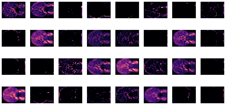
How about the next convolutional layer? Remember: it should get more abstract!

show_activation('conv2d_4')

/var/folders/61/0lj9r7px3k52gv9yfyx6ky300000gn/T/ipykernel_52465/4057567175.py:21: MatplotlibDeprecationWarning:

Passing non-integers as three-element position specification is deprecated since 3.3 and will be removed two minor releases later.

../../../_images/DL_build_train_159_1.png

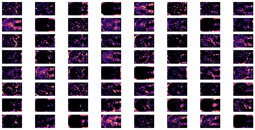
And finally, the last convolutional layer:

show_activation('conv2d_5')

/var/folders/61/0lj9r7px3k52gv9yfyx6ky300000gn/T/ipykernel_52465/4057567175.py:21: MatplotlibDeprecationWarning:

Passing non-integers as three-element position specification is deprecated since 3.3 and will be removed two minor releases later.

../../../_images/DL_build_train_161_1.png

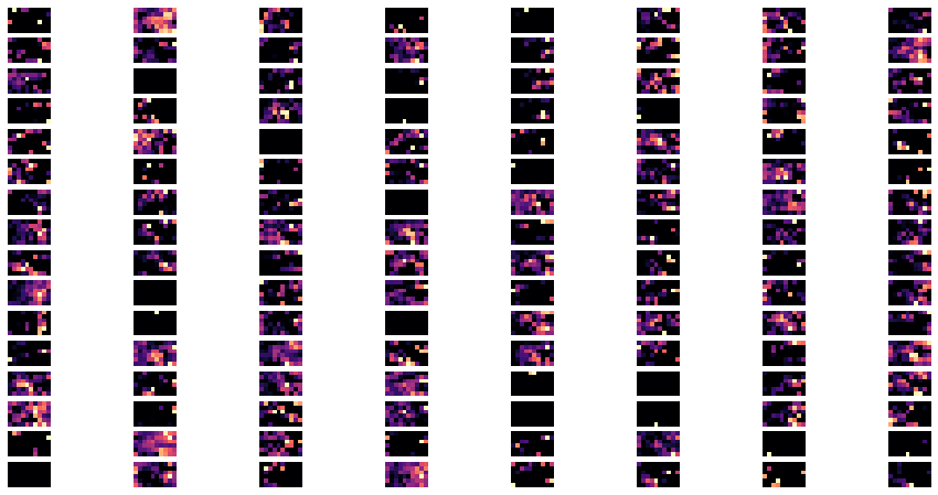
Fancy, eh? How would describe this and do you think this helpful to understand what our ANN does?

Are there any more options that come to your mind how we can further evaluate our (pre-) trained ANN?

How about going back to the basic concepts and thinking about generalization? We know how our ANN performs in the hold-out test set of our dataset but what about completely different data? Data that varies more or less prominently in several aspects (think about what these aspects could be)? Remember: we’re interested in invariant representations and thus, if our ANN really learned something generalizable. In turn, we should be able to feed it a different dataset with diverging specifics and yet obtain sensible outcomes, i.e. a good performance.

`Generalization`¶

That being said: let’s bring back an old friend, our example dataset from the “classic” machine learning part. It’s also a resting state fMRI dataset, but different in terms of participants, data acquisition sequence, etc. . Previously, we worked with vectorized connectivity matrices but now we need the fMRI volumes/images. Thus, we need to download them first:

import urllib.request

url = 'https://www.dropbox.com/s/73xlwtcochbytpv/dataset_ML_eval.nii.gz?dl=1'
urllib.request.urlretrieve(url, 'dataest_ML_eval.nii.gz')

('dataest_ML_eval.nii.gz', <http.client.HTTPMessage at 0x7fe3263e0130>)

As usual, let’s load them and have a brief look:

dataset_eval = nb.load('dataest_ML_eval.nii.gz')
dataset_eval.shape

(50, 59, 50, 155)

dataset_eval.orthoview()

<OrthoSlicer3D: dataest_ML_eval.nii.gz (50, 59, 50, 155)>

../../../_images/DL_build_train_169_1.png

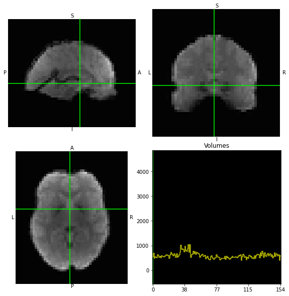
To once more accommodate the restricted time and resource situation, we didn’t include the entire dataset, but only the middle volume of each participants’ fMRI images.

As mentioned several times before: one of the crucial parts of re-using existing ANNs on new data is to bring the new data into the format that is expected by the ANN, i.e. the input layer. Thus, we need to prepare the data a bit… (Please note: this is something you’ll have to do as well when re-using existing ANNs with your data and therefore always make sure to consult the respective documentation and/or respective publication.)

Going back to the beginning of this section, we remember that our input layer expects the data in the form of samples, x, y, z and that we submitted only a couple of slices of the image after we rotated it. Let’s just re-use the respective code (Please note: Always be careful with that and check things more than once, copy+paste can be very dangerous!)

from nilearn.image import resample_to_img

# we re-load the initial dataset here
data = nb.load('dataest_ML.nii.gz')

# we resample the images our new dataset to those of the initial dataset
dataset_eval_resmp = resample_to_img(dataset_eval, data)

# we rotate our new dataset
dataset_eval_affine = nb.Nifti1Image(dataset_eval_resmp.get_fdata(), new_affine)
dataset_eval_rot = resample_img(dataset_eval_affine, data.affine, interpolation='continuous')

# we get the slices of our new dataset
dataset_eval_slab = dataset_eval_rot.slicer[..., 12:15, :]

# we change the dimensions of our new dataset's slab
data_eval = np.rollaxis(dataset_eval_slab.get_fdata(), 3, 0)
data_eval.shape

(155, 40, 56, 3)

That looks about right, but we can also make sure that the dimensions of our initial dataset and our new dataset fit:

data.shape[1:] 

(51, 41, 384)

data_eval.shape[1:]

(40, 56, 3)

Great, now we can already put our ANN back to work and let it predict the new dataset:

dataset_eval_y_pred = np.argmax(model.predict(X_test), axis=1)
dataset_eval_y_pred

array([0, 1, 1, 1, 1, 0, 0, 0, 0, 1, 1, 1, 1, 0, 0, 0, 0, 1, 1, 1, 1, 0,
       0, 0, 0, 1, 1, 1, 1, 0, 0, 0, 0, 1, 1, 1, 0, 0, 0, 0, 0, 1, 0, 1,
       1, 0, 0, 0, 0, 1, 1, 1, 0, 1, 0, 1, 0, 1, 1, 1, 1, 0, 0, 0, 0, 1,
       0, 1, 1, 0, 0, 0, 0, 0, 1, 0, 0])

Ok, worked like a charm! However, how can we evaluate the ANN’s performance on the new dataset?

Ha, gotcha: We simply can not! The new dataset we were investigating doesn’t have any labels useful for the task our ANN was built and trained to do, that is the recognition and distinction of eyes open vs. eyes closed. It will of course still work, i.e. predict, because it doesn’t know that but we just have no option to evaluate its performance.

_{^{_{^{^{https://c.tenor.com/W3ThqxOhD-cAAAAC/gotcha-fooled-you.gif}}}}}

However….we do have labels for this new/old dataset, namely for the task(s) we tried during the “classic” machine learning part: predicting a participant’s age or age group. So what we theoretically could do is to assume that the representations our ANN learned will also help it to achieve this new task. Does this ring a bell?

Transfer learning¶

That’s right folks: it’s about transfer learning. The idea would be that the representations learned by our ANN to recognize and distinguish eyes open vs. eyes closed will also help it to recognize and distinguish age groups. Please note: we’re leaving the reasonableness behind here as we want to showcase transfer learning but can you think of potentially more feasible transfer learning problems?

Thinking back to the previous section, we talked about how transfer learning works in theory: we “simply” re-train the output layer or several layers for the new task. In practice this means we will remove the learned weights of these layers and "freeze" the other ones, thus only the first will be updated based on the new task and the corresponding loss function and optimization.

Question: why re-train at all and not just simply providing the new data and respective labels?

Ok, but how do we do this transfer learning? At first, we will get the labels in order to define our training and test set.

import pandas as pd
information = pd.read_csv('participants.csv')
information.head(n=5)

	participant_id	Age	AgeGroup	Child_Adult	Gender	Handedness
0	sub-pixar123	27.06	Adult	adult	F	R
1	sub-pixar124	33.44	Adult	adult	M	R
2	sub-pixar125	31.00	Adult	adult	M	R
3	sub-pixar126	19.00	Adult	adult	F	R
4	sub-pixar127	23.00	Adult	adult	F	R

Y_cat = information['Child_Adult']
Y_cat.describe()

count       155
unique        2
top       child
freq        122
Name: Child_Adult, dtype: object

It’s been a while, so let’s plot them:

import plotly.express as px
from IPython.core.display import display, HTML
from plotly.offline import init_notebook_mode, plot

fig = px.histogram(Y_cat, marginal='box', template='plotly_white')

fig.update_layout(showlegend=False, width=800, height=800)
init_notebook_mode(connected=True)

#fig.show()

plot(fig, filename = 'labels_dl_eval.html')
display(HTML('labels_dl_eval.html'))

Alright, creating training and test datasets is old news for you by now:

age_class = information.loc[Y_cat.index,'Child_Adult']

Y_cat = Y_cat =='adult'

X_train, X_test, y_train, y_test = train_test_split(data_eval, Y_cat, random_state=0, shuffle=True, stratify=age_class)

print('Shapes of X:', X_train.shape, X_test.shape)
print('Shapes of y:', y_train.shape, y_test.shape)

Shapes of X: (116, 40, 56, 3) (39, 40, 56, 3)
Shapes of y: (116,) (39,)

Now we will save our ANN to have its architecture and especially weights on file.

model.save('ANN_eyes')

2021-09-21 15:44:05.296468: W tensorflow/python/util/util.cc:348] Sets are not currently considered sequences, but this may change in the future, so consider avoiding using them.

INFO:tensorflow:Assets written to: ANN_eyes/assets

We could also just have saved the weights like so:

model.save_weights('ANN_eyes_weights')

Depending on the model and the way folks provided it, you might encounter several of these and other options when you want to use pre-trained models.

Now it’s time to define our new ANN via basically loading the one we just saved into a new instance:

from tensorflow.keras.models import load_model

model_age = load_model('ANN_eyes')

We can easily make sure the ANN looks as expected:

model_age.summary()

Model: "sequential_1"
_________________________________________________________________
Layer (type)                 Output Shape              Param #   
=================================================================
conv2d_3 (Conv2D)            (None, 38, 54, 32)        896       
_________________________________________________________________
batch_normalization_6 (Batch (None, 38, 54, 32)        128       
_________________________________________________________________
max_pooling2d_3 (MaxPooling2 (None, 19, 27, 32)        0         
_________________________________________________________________
conv2d_4 (Conv2D)            (None, 17, 25, 64)        18496     
_________________________________________________________________
batch_normalization_7 (Batch (None, 17, 25, 64)        256       
_________________________________________________________________
max_pooling2d_4 (MaxPooling2 (None, 8, 12, 64)         0         
_________________________________________________________________
conv2d_5 (Conv2D)            (None, 6, 10, 128)        73856     
_________________________________________________________________
batch_normalization_8 (Batch (None, 6, 10, 128)        512       
_________________________________________________________________
max_pooling2d_5 (MaxPooling2 (None, 3, 5, 128)         0         
_________________________________________________________________
flatten_1 (Flatten)          (None, 1920)              0         
_________________________________________________________________
dropout_4 (Dropout)          (None, 1920)              0         
_________________________________________________________________
dense_4 (Dense)              (None, 1024)              1967104   
_________________________________________________________________
batch_normalization_9 (Batch (None, 1024)              4096      
_________________________________________________________________
dropout_5 (Dropout)          (None, 1024)              0         
_________________________________________________________________
dense_5 (Dense)              (None, 256)               262400    
_________________________________________________________________
batch_normalization_10 (Batc (None, 256)               1024      
_________________________________________________________________
dropout_6 (Dropout)          (None, 256)               0         
_________________________________________________________________
dense_6 (Dense)              (None, 64)                16448     
_________________________________________________________________
batch_normalization_11 (Batc (None, 64)                256       
_________________________________________________________________
dropout_7 (Dropout)          (None, 64)                0         
_________________________________________________________________
dense_7 (Dense)              (None, 2)                 130       
=================================================================
Total params: 2,345,602
Trainable params: 2,342,466
Non-trainable params: 3,136
_________________________________________________________________

Check, that looks as it should. What follows is the central part: we tell the ANN that only its last, i.e. output layer, will be trainable, i.e. capable of updating its weights with the others remaining the same:

model_age.load_weights('ANN_eyes_weights')

for layer in model_age.layers[:-1]:
    layer.trainable = False

model_age.summary()

Model: "sequential_1"
_________________________________________________________________
Layer (type)                 Output Shape              Param #   
=================================================================
conv2d_3 (Conv2D)            (None, 38, 54, 32)        896       
_________________________________________________________________
batch_normalization_6 (Batch (None, 38, 54, 32)        128       
_________________________________________________________________
max_pooling2d_3 (MaxPooling2 (None, 19, 27, 32)        0         
_________________________________________________________________
conv2d_4 (Conv2D)            (None, 17, 25, 64)        18496     
_________________________________________________________________
batch_normalization_7 (Batch (None, 17, 25, 64)        256       
_________________________________________________________________
max_pooling2d_4 (MaxPooling2 (None, 8, 12, 64)         0         
_________________________________________________________________
conv2d_5 (Conv2D)            (None, 6, 10, 128)        73856     
_________________________________________________________________
batch_normalization_8 (Batch (None, 6, 10, 128)        512       
_________________________________________________________________
max_pooling2d_5 (MaxPooling2 (None, 3, 5, 128)         0         
_________________________________________________________________
flatten_1 (Flatten)          (None, 1920)              0         
_________________________________________________________________
dropout_4 (Dropout)          (None, 1920)              0         
_________________________________________________________________
dense_4 (Dense)              (None, 1024)              1967104   
_________________________________________________________________
batch_normalization_9 (Batch (None, 1024)              4096      
_________________________________________________________________
dropout_5 (Dropout)          (None, 1024)              0         
_________________________________________________________________
dense_5 (Dense)              (None, 256)               262400    
_________________________________________________________________
batch_normalization_10 (Batc (None, 256)               1024      
_________________________________________________________________
dropout_6 (Dropout)          (None, 256)               0         
_________________________________________________________________
dense_6 (Dense)              (None, 64)                16448     
_________________________________________________________________
batch_normalization_11 (Batc (None, 64)                256       
_________________________________________________________________
dropout_7 (Dropout)          (None, 64)                0         
_________________________________________________________________
dense_7 (Dense)              (None, 2)                 130       
=================================================================
Total params: 2,345,602
Trainable params: 130
Non-trainable params: 2,345,472
_________________________________________________________________

The rest of steps are identical to the first time we utilized our ANN: building via the .compile() function, training via the .fit() function and then inspecting its performance. We will keep the same metric, loss function and optimizer as before:

model_age.compile(loss='sparse_categorical_crossentropy',
              optimizer='adam', 
              metrics=['accuracy'])

The same holds true for number of epochs, batch size and the validation split, logging everything to use tensorboard again after the training:

logdir = os.path.join("logs_age", datetime.datetime.now().strftime("%Y%m%d-%H%M%S"))
tensorboard_callback = tf.keras.callbacks.TensorBoard(logdir, histogram_freq=1)

%time fit_age = model_age.fit(X_train, y_train, epochs=125, batch_size=32, validation_split=0.2, callbacks=[tensorboard_callback])

Epoch 1/125
3/3 [==============================] - ETA: 0s - loss: 887.8113 - accuracy: 0.4783

2021-09-21 15:44:50.489680: I tensorflow/core/profiler/lib/profiler_session.cc:131] Profiler session initializing.
2021-09-21 15:44:50.489693: I tensorflow/core/profiler/lib/profiler_session.cc:146] Profiler session started.
2021-09-21 15:44:50.570161: I tensorflow/core/profiler/lib/profiler_session.cc:66] Profiler session collecting data.
2021-09-21 15:44:50.571914: I tensorflow/core/profiler/lib/profiler_session.cc:164] Profiler session tear down.
2021-09-21 15:44:50.573151: I tensorflow/core/profiler/rpc/client/save_profile.cc:136] Creating directory: logs_age/20210921-154408/train/plugins/profile/2021_09_21_15_44_50

2021-09-21 15:44:50.574030: I tensorflow/core/profiler/rpc/client/save_profile.cc:142] Dumped gzipped tool data for trace.json.gz to logs_age/20210921-154408/train/plugins/profile/2021_09_21_15_44_50/Peers-MBP.trace.json.gz
2021-09-21 15:44:50.576003: I tensorflow/core/profiler/rpc/client/save_profile.cc:136] Creating directory: logs_age/20210921-154408/train/plugins/profile/2021_09_21_15_44_50

2021-09-21 15:44:50.576212: I tensorflow/core/profiler/rpc/client/save_profile.cc:142] Dumped gzipped tool data for memory_profile.json.gz to logs_age/20210921-154408/train/plugins/profile/2021_09_21_15_44_50/Peers-MBP.memory_profile.json.gz
2021-09-21 15:44:50.576985: I tensorflow/core/profiler/rpc/client/capture_profile.cc:251] Creating directory: logs_age/20210921-154408/train/plugins/profile/2021_09_21_15_44_50
Dumped tool data for xplane.pb to logs_age/20210921-154408/train/plugins/profile/2021_09_21_15_44_50/Peers-MBP.xplane.pb
Dumped tool data for overview_page.pb to logs_age/20210921-154408/train/plugins/profile/2021_09_21_15_44_50/Peers-MBP.overview_page.pb
Dumped tool data for input_pipeline.pb to logs_age/20210921-154408/train/plugins/profile/2021_09_21_15_44_50/Peers-MBP.input_pipeline.pb
Dumped tool data for tensorflow_stats.pb to logs_age/20210921-154408/train/plugins/profile/2021_09_21_15_44_50/Peers-MBP.tensorflow_stats.pb
Dumped tool data for kernel_stats.pb to logs_age/20210921-154408/train/plugins/profile/2021_09_21_15_44_50/Peers-MBP.kernel_stats.pb

3/3 [==============================] - 1s 173ms/step - loss: 887.8113 - accuracy: 0.4783 - val_loss: 88.9316 - val_accuracy: 0.7083
Epoch 2/125
3/3 [==============================] - 0s 36ms/step - loss: 584.9210 - accuracy: 0.5326 - val_loss: 83.6666 - val_accuracy: 0.6250
Epoch 3/125
3/3 [==============================] - 0s 36ms/step - loss: 829.7230 - accuracy: 0.4457 - val_loss: 79.8900 - val_accuracy: 0.6250
Epoch 4/125
3/3 [==============================] - 0s 34ms/step - loss: 781.0987 - accuracy: 0.5000 - val_loss: 75.8917 - val_accuracy: 0.6250
Epoch 5/125
3/3 [==============================] - 0s 33ms/step - loss: 527.5601 - accuracy: 0.5652 - val_loss: 72.2877 - val_accuracy: 0.5833
Epoch 6/125
3/3 [==============================] - 0s 34ms/step - loss: 720.2014 - accuracy: 0.5543 - val_loss: 71.0733 - val_accuracy: 0.6250
Epoch 7/125
3/3 [==============================] - 0s 34ms/step - loss: 560.6887 - accuracy: 0.5761 - val_loss: 70.5163 - val_accuracy: 0.6250
Epoch 8/125
3/3 [==============================] - 0s 35ms/step - loss: 537.1358 - accuracy: 0.6087 - val_loss: 72.2585 - val_accuracy: 0.7083
Epoch 9/125
3/3 [==============================] - 0s 34ms/step - loss: 646.9361 - accuracy: 0.6304 - val_loss: 74.9470 - val_accuracy: 0.7083
Epoch 10/125
3/3 [==============================] - 0s 34ms/step - loss: 437.4638 - accuracy: 0.6413 - val_loss: 77.1222 - val_accuracy: 0.7083
Epoch 11/125
3/3 [==============================] - 0s 35ms/step - loss: 446.1407 - accuracy: 0.6957 - val_loss: 79.3083 - val_accuracy: 0.6667
Epoch 12/125
3/3 [==============================] - 0s 34ms/step - loss: 441.9286 - accuracy: 0.6957 - val_loss: 81.6235 - val_accuracy: 0.6667
Epoch 13/125
3/3 [==============================] - 0s 32ms/step - loss: 399.8640 - accuracy: 0.7174 - val_loss: 83.0715 - val_accuracy: 0.6667
Epoch 14/125
3/3 [==============================] - 0s 34ms/step - loss: 337.0713 - accuracy: 0.6630 - val_loss: 84.1901 - val_accuracy: 0.6667
Epoch 15/125
3/3 [==============================] - 0s 33ms/step - loss: 431.2654 - accuracy: 0.6848 - val_loss: 85.4378 - val_accuracy: 0.6667
Epoch 16/125
3/3 [==============================] - 0s 34ms/step - loss: 410.9785 - accuracy: 0.6304 - val_loss: 86.4693 - val_accuracy: 0.6667
Epoch 17/125
3/3 [==============================] - 0s 34ms/step - loss: 427.2539 - accuracy: 0.7174 - val_loss: 87.3070 - val_accuracy: 0.6667
Epoch 18/125
3/3 [==============================] - 0s 33ms/step - loss: 356.3279 - accuracy: 0.6522 - val_loss: 88.3478 - val_accuracy: 0.7083
Epoch 19/125
3/3 [==============================] - 0s 33ms/step - loss: 428.8806 - accuracy: 0.6630 - val_loss: 90.7753 - val_accuracy: 0.7500
Epoch 20/125
3/3 [==============================] - 0s 33ms/step - loss: 503.8941 - accuracy: 0.6413 - val_loss: 92.7706 - val_accuracy: 0.7500
Epoch 21/125
3/3 [==============================] - 0s 34ms/step - loss: 621.1743 - accuracy: 0.5761 - val_loss: 95.0197 - val_accuracy: 0.7083
Epoch 22/125
3/3 [==============================] - 0s 34ms/step - loss: 377.0852 - accuracy: 0.7065 - val_loss: 97.2071 - val_accuracy: 0.7083
Epoch 23/125
3/3 [==============================] - 0s 35ms/step - loss: 281.5693 - accuracy: 0.7065 - val_loss: 98.5911 - val_accuracy: 0.7083
Epoch 24/125
3/3 [==============================] - 0s 33ms/step - loss: 561.8777 - accuracy: 0.6522 - val_loss: 99.2645 - val_accuracy: 0.7083
Epoch 25/125
3/3 [==============================] - 0s 34ms/step - loss: 342.1421 - accuracy: 0.7500 - val_loss: 99.9534 - val_accuracy: 0.7083
Epoch 26/125
3/3 [==============================] - 0s 35ms/step - loss: 285.3293 - accuracy: 0.7283 - val_loss: 100.0415 - val_accuracy: 0.7083
Epoch 27/125
3/3 [==============================] - 0s 36ms/step - loss: 235.7388 - accuracy: 0.6957 - val_loss: 101.2710 - val_accuracy: 0.7083
Epoch 28/125
3/3 [==============================] - 0s 34ms/step - loss: 426.4846 - accuracy: 0.6848 - val_loss: 101.7703 - val_accuracy: 0.7083
Epoch 29/125
3/3 [==============================] - 0s 34ms/step - loss: 308.6684 - accuracy: 0.7065 - val_loss: 102.8744 - val_accuracy: 0.7083
Epoch 30/125
3/3 [==============================] - 0s 32ms/step - loss: 374.2005 - accuracy: 0.6848 - val_loss: 104.2225 - val_accuracy: 0.7083
Epoch 31/125
3/3 [==============================] - 0s 34ms/step - loss: 373.1317 - accuracy: 0.6630 - val_loss: 106.2061 - val_accuracy: 0.7083
Epoch 32/125
3/3 [==============================] - 0s 33ms/step - loss: 364.0777 - accuracy: 0.6957 - val_loss: 107.6613 - val_accuracy: 0.7083
Epoch 33/125
3/3 [==============================] - 0s 33ms/step - loss: 368.9847 - accuracy: 0.7065 - val_loss: 108.9394 - val_accuracy: 0.7083
Epoch 34/125
3/3 [==============================] - 0s 34ms/step - loss: 373.8293 - accuracy: 0.6848 - val_loss: 110.0365 - val_accuracy: 0.7083
Epoch 35/125
3/3 [==============================] - 0s 35ms/step - loss: 516.2195 - accuracy: 0.7174 - val_loss: 109.9914 - val_accuracy: 0.7083
Epoch 36/125
3/3 [==============================] - 0s 33ms/step - loss: 327.7397 - accuracy: 0.7174 - val_loss: 110.2708 - val_accuracy: 0.7083
Epoch 37/125
3/3 [==============================] - 0s 33ms/step - loss: 227.8714 - accuracy: 0.7500 - val_loss: 109.8888 - val_accuracy: 0.7083
Epoch 38/125
3/3 [==============================] - 0s 33ms/step - loss: 330.5888 - accuracy: 0.7283 - val_loss: 109.3391 - val_accuracy: 0.7083
Epoch 39/125
3/3 [==============================] - 0s 34ms/step - loss: 382.6850 - accuracy: 0.7391 - val_loss: 108.8459 - val_accuracy: 0.7083
Epoch 40/125
3/3 [==============================] - 0s 34ms/step - loss: 379.6105 - accuracy: 0.7717 - val_loss: 107.7057 - val_accuracy: 0.7083
Epoch 41/125
3/3 [==============================] - 0s 35ms/step - loss: 413.2135 - accuracy: 0.7609 - val_loss: 106.2207 - val_accuracy: 0.7083
Epoch 42/125
3/3 [==============================] - 0s 32ms/step - loss: 281.8456 - accuracy: 0.7500 - val_loss: 104.2112 - val_accuracy: 0.7083
Epoch 43/125
3/3 [==============================] - 0s 33ms/step - loss: 378.3797 - accuracy: 0.6848 - val_loss: 102.1119 - val_accuracy: 0.7083
Epoch 44/125
3/3 [==============================] - 0s 33ms/step - loss: 266.3713 - accuracy: 0.7283 - val_loss: 99.8318 - val_accuracy: 0.7083
Epoch 45/125
3/3 [==============================] - 0s 33ms/step - loss: 293.1965 - accuracy: 0.7174 - val_loss: 98.2014 - val_accuracy: 0.7083
Epoch 46/125
3/3 [==============================] - 0s 33ms/step - loss: 503.1194 - accuracy: 0.6957 - val_loss: 96.0998 - val_accuracy: 0.7083
Epoch 47/125
3/3 [==============================] - 0s 33ms/step - loss: 269.9908 - accuracy: 0.6957 - val_loss: 94.0089 - val_accuracy: 0.7083
Epoch 48/125
3/3 [==============================] - 0s 33ms/step - loss: 220.6680 - accuracy: 0.7065 - val_loss: 92.3736 - val_accuracy: 0.7083
Epoch 49/125
3/3 [==============================] - 0s 35ms/step - loss: 438.9058 - accuracy: 0.6522 - val_loss: 91.0415 - val_accuracy: 0.7083
Epoch 50/125
3/3 [==============================] - 0s 35ms/step - loss: 242.7601 - accuracy: 0.6739 - val_loss: 90.1206 - val_accuracy: 0.7083
Epoch 51/125
3/3 [==============================] - 0s 35ms/step - loss: 165.6752 - accuracy: 0.7609 - val_loss: 88.9573 - val_accuracy: 0.7083
Epoch 52/125
3/3 [==============================] - 0s 37ms/step - loss: 301.5461 - accuracy: 0.6739 - val_loss: 87.3599 - val_accuracy: 0.7083
Epoch 53/125
3/3 [==============================] - 0s 34ms/step - loss: 230.7517 - accuracy: 0.7391 - val_loss: 85.6637 - val_accuracy: 0.7083
Epoch 54/125
3/3 [==============================] - 0s 35ms/step - loss: 246.6116 - accuracy: 0.7283 - val_loss: 83.7182 - val_accuracy: 0.7083
Epoch 55/125
3/3 [==============================] - 0s 35ms/step - loss: 348.6924 - accuracy: 0.6957 - val_loss: 80.9762 - val_accuracy: 0.7083
Epoch 56/125
3/3 [==============================] - 0s 34ms/step - loss: 232.9588 - accuracy: 0.7500 - val_loss: 78.6683 - val_accuracy: 0.7083
Epoch 57/125
3/3 [==============================] - 0s 41ms/step - loss: 225.1206 - accuracy: 0.7391 - val_loss: 76.7163 - val_accuracy: 0.7083
Epoch 58/125
3/3 [==============================] - 0s 40ms/step - loss: 152.9310 - accuracy: 0.7174 - val_loss: 75.4419 - val_accuracy: 0.7083
Epoch 59/125
3/3 [==============================] - 0s 34ms/step - loss: 251.3504 - accuracy: 0.7391 - val_loss: 73.8538 - val_accuracy: 0.7083
Epoch 60/125
3/3 [==============================] - 0s 36ms/step - loss: 272.5712 - accuracy: 0.6957 - val_loss: 72.5380 - val_accuracy: 0.7083
Epoch 61/125
3/3 [==============================] - 0s 40ms/step - loss: 164.9235 - accuracy: 0.7391 - val_loss: 72.0039 - val_accuracy: 0.7083
Epoch 62/125
3/3 [==============================] - 0s 36ms/step - loss: 212.9399 - accuracy: 0.6957 - val_loss: 71.4572 - val_accuracy: 0.7083
Epoch 63/125
3/3 [==============================] - 0s 34ms/step - loss: 167.1405 - accuracy: 0.7500 - val_loss: 70.5901 - val_accuracy: 0.7083
Epoch 64/125
3/3 [==============================] - 0s 37ms/step - loss: 232.2369 - accuracy: 0.7391 - val_loss: 69.0886 - val_accuracy: 0.7083
Epoch 65/125
3/3 [==============================] - 0s 36ms/step - loss: 206.6786 - accuracy: 0.7065 - val_loss: 67.4554 - val_accuracy: 0.7083
Epoch 66/125
3/3 [==============================] - 0s 35ms/step - loss: 233.4057 - accuracy: 0.7717 - val_loss: 64.3124 - val_accuracy: 0.7083
Epoch 67/125
3/3 [==============================] - 0s 34ms/step - loss: 232.0701 - accuracy: 0.6739 - val_loss: 61.8038 - val_accuracy: 0.7083
Epoch 68/125
3/3 [==============================] - 0s 35ms/step - loss: 192.2046 - accuracy: 0.6957 - val_loss: 58.7224 - val_accuracy: 0.7083
Epoch 69/125
3/3 [==============================] - 0s 37ms/step - loss: 223.4950 - accuracy: 0.6630 - val_loss: 56.7811 - val_accuracy: 0.7083
Epoch 70/125
3/3 [==============================] - 0s 43ms/step - loss: 224.7231 - accuracy: 0.7065 - val_loss: 54.6440 - val_accuracy: 0.7083
Epoch 71/125
3/3 [==============================] - 0s 50ms/step - loss: 169.7887 - accuracy: 0.7717 - val_loss: 52.1129 - val_accuracy: 0.7083
Epoch 72/125
3/3 [==============================] - 0s 34ms/step - loss: 249.5327 - accuracy: 0.6630 - val_loss: 50.0436 - val_accuracy: 0.7083
Epoch 73/125
3/3 [==============================] - 0s 35ms/step - loss: 219.2719 - accuracy: 0.7283 - val_loss: 49.0691 - val_accuracy: 0.7083
Epoch 74/125
3/3 [==============================] - 0s 36ms/step - loss: 198.5319 - accuracy: 0.7283 - val_loss: 48.4191 - val_accuracy: 0.7083
Epoch 75/125
3/3 [==============================] - 0s 35ms/step - loss: 213.9902 - accuracy: 0.7500 - val_loss: 47.2782 - val_accuracy: 0.7083
Epoch 76/125
3/3 [==============================] - 0s 34ms/step - loss: 190.8896 - accuracy: 0.6630 - val_loss: 45.9932 - val_accuracy: 0.7083
Epoch 77/125
3/3 [==============================] - 0s 35ms/step - loss: 193.1330 - accuracy: 0.7283 - val_loss: 43.6197 - val_accuracy: 0.7083
Epoch 78/125
3/3 [==============================] - 0s 34ms/step - loss: 165.7709 - accuracy: 0.7174 - val_loss: 41.3496 - val_accuracy: 0.7083
Epoch 79/125
3/3 [==============================] - 0s 34ms/step - loss: 75.8008 - accuracy: 0.7826 - val_loss: 39.4995 - val_accuracy: 0.7083
Epoch 80/125
3/3 [==============================] - 0s 33ms/step - loss: 67.7243 - accuracy: 0.7609 - val_loss: 37.9464 - val_accuracy: 0.7083
Epoch 81/125
3/3 [==============================] - 0s 34ms/step - loss: 147.3556 - accuracy: 0.6957 - val_loss: 37.1398 - val_accuracy: 0.7083
Epoch 82/125
3/3 [==============================] - 0s 34ms/step - loss: 242.2355 - accuracy: 0.7283 - val_loss: 35.4815 - val_accuracy: 0.7083
Epoch 83/125
3/3 [==============================] - 0s 34ms/step - loss: 151.1039 - accuracy: 0.6957 - val_loss: 34.4667 - val_accuracy: 0.7083
Epoch 84/125
3/3 [==============================] - 0s 33ms/step - loss: 169.7370 - accuracy: 0.7065 - val_loss: 33.0668 - val_accuracy: 0.7083
Epoch 85/125
3/3 [==============================] - 0s 34ms/step - loss: 120.2526 - accuracy: 0.7500 - val_loss: 31.2726 - val_accuracy: 0.7083
Epoch 86/125
3/3 [==============================] - 0s 34ms/step - loss: 60.2437 - accuracy: 0.7609 - val_loss: 30.8126 - val_accuracy: 0.7083
Epoch 87/125
3/3 [==============================] - 0s 35ms/step - loss: 136.5704 - accuracy: 0.7283 - val_loss: 29.6757 - val_accuracy: 0.7083
Epoch 88/125
3/3 [==============================] - 0s 34ms/step - loss: 99.9262 - accuracy: 0.7717 - val_loss: 28.2337 - val_accuracy: 0.7083
Epoch 89/125
3/3 [==============================] - 0s 35ms/step - loss: 83.0590 - accuracy: 0.7283 - val_loss: 26.1691 - val_accuracy: 0.7083
Epoch 90/125
3/3 [==============================] - 0s 34ms/step - loss: 145.5207 - accuracy: 0.6087 - val_loss: 25.6922 - val_accuracy: 0.7083
Epoch 91/125
3/3 [==============================] - 0s 36ms/step - loss: 108.2622 - accuracy: 0.6739 - val_loss: 26.6134 - val_accuracy: 0.7083
Epoch 92/125
3/3 [==============================] - 0s 34ms/step - loss: 126.7695 - accuracy: 0.6848 - val_loss: 27.9427 - val_accuracy: 0.7083
Epoch 93/125
3/3 [==============================] - 0s 48ms/step - loss: 88.8239 - accuracy: 0.8043 - val_loss: 28.3391 - val_accuracy: 0.7083
Epoch 94/125
3/3 [==============================] - 0s 35ms/step - loss: 109.6099 - accuracy: 0.6739 - val_loss: 28.0788 - val_accuracy: 0.7083
Epoch 95/125
3/3 [==============================] - 0s 33ms/step - loss: 75.6291 - accuracy: 0.7935 - val_loss: 26.4664 - val_accuracy: 0.7083
Epoch 96/125
3/3 [==============================] - 0s 34ms/step - loss: 85.0009 - accuracy: 0.7174 - val_loss: 24.6660 - val_accuracy: 0.7083
Epoch 97/125
3/3 [==============================] - 0s 34ms/step - loss: 112.7472 - accuracy: 0.6848 - val_loss: 23.2306 - val_accuracy: 0.7083
Epoch 98/125
3/3 [==============================] - 0s 34ms/step - loss: 85.4779 - accuracy: 0.7065 - val_loss: 22.2507 - val_accuracy: 0.7083
Epoch 99/125
3/3 [==============================] - 0s 33ms/step - loss: 109.3718 - accuracy: 0.7174 - val_loss: 22.1949 - val_accuracy: 0.7083
Epoch 100/125
3/3 [==============================] - 0s 33ms/step - loss: 77.3136 - accuracy: 0.7391 - val_loss: 22.8056 - val_accuracy: 0.7083
Epoch 101/125
3/3 [==============================] - 0s 33ms/step - loss: 78.8479 - accuracy: 0.7935 - val_loss: 22.1076 - val_accuracy: 0.7083
Epoch 102/125
3/3 [==============================] - 0s 37ms/step - loss: 64.8638 - accuracy: 0.7609 - val_loss: 20.9219 - val_accuracy: 0.7083
Epoch 103/125
3/3 [==============================] - 0s 35ms/step - loss: 88.3198 - accuracy: 0.7174 - val_loss: 20.2806 - val_accuracy: 0.7083
Epoch 104/125
3/3 [==============================] - 0s 34ms/step - loss: 76.5946 - accuracy: 0.7609 - val_loss: 19.3569 - val_accuracy: 0.7083
Epoch 105/125
3/3 [==============================] - 0s 33ms/step - loss: 101.5569 - accuracy: 0.7391 - val_loss: 17.8958 - val_accuracy: 0.7083
Epoch 106/125
3/3 [==============================] - 0s 32ms/step - loss: 70.3167 - accuracy: 0.7174 - val_loss: 18.2392 - val_accuracy: 0.7083
Epoch 107/125
3/3 [==============================] - 0s 33ms/step - loss: 70.2217 - accuracy: 0.7826 - val_loss: 16.7997 - val_accuracy: 0.7083
Epoch 108/125
3/3 [==============================] - 0s 34ms/step - loss: 75.9625 - accuracy: 0.7065 - val_loss: 15.1137 - val_accuracy: 0.7083
Epoch 109/125
3/3 [==============================] - 0s 34ms/step - loss: 49.0417 - accuracy: 0.7500 - val_loss: 14.4519 - val_accuracy: 0.7083
Epoch 110/125
3/3 [==============================] - 0s 34ms/step - loss: 70.8944 - accuracy: 0.7500 - val_loss: 13.5672 - val_accuracy: 0.7083
Epoch 111/125
3/3 [==============================] - 0s 34ms/step - loss: 59.8224 - accuracy: 0.7391 - val_loss: 11.3995 - val_accuracy: 0.6667
Epoch 112/125
3/3 [==============================] - 0s 34ms/step - loss: 62.5213 - accuracy: 0.6522 - val_loss: 9.7859 - val_accuracy: 0.6667
Epoch 113/125
3/3 [==============================] - 0s 34ms/step - loss: 67.8922 - accuracy: 0.7283 - val_loss: 8.8819 - val_accuracy: 0.6667
Epoch 114/125
3/3 [==============================] - 0s 33ms/step - loss: 47.9223 - accuracy: 0.7717 - val_loss: 7.6508 - val_accuracy: 0.6667
Epoch 115/125
3/3 [==============================] - 0s 33ms/step - loss: 37.6088 - accuracy: 0.6630 - val_loss: 6.3876 - val_accuracy: 0.7083
Epoch 116/125
3/3 [==============================] - 0s 33ms/step - loss: 42.7875 - accuracy: 0.7391 - val_loss: 5.7816 - val_accuracy: 0.7500
Epoch 117/125
3/3 [==============================] - 0s 35ms/step - loss: 42.9551 - accuracy: 0.7065 - val_loss: 5.3477 - val_accuracy: 0.6667
Epoch 118/125
3/3 [==============================] - 0s 34ms/step - loss: 49.5616 - accuracy: 0.6848 - val_loss: 4.9940 - val_accuracy: 0.7083
Epoch 119/125
3/3 [==============================] - 0s 34ms/step - loss: 46.0876 - accuracy: 0.6304 - val_loss: 5.2064 - val_accuracy: 0.7083
Epoch 120/125
3/3 [==============================] - 0s 33ms/step - loss: 56.6767 - accuracy: 0.6848 - val_loss: 6.7024 - val_accuracy: 0.6667
Epoch 121/125
3/3 [==============================] - 0s 34ms/step - loss: 31.4218 - accuracy: 0.7826 - val_loss: 7.4837 - val_accuracy: 0.7083
Epoch 122/125
3/3 [==============================] - 0s 36ms/step - loss: 41.5343 - accuracy: 0.6848 - val_loss: 8.0882 - val_accuracy: 0.7083
Epoch 123/125
3/3 [==============================] - 0s 33ms/step - loss: 42.2206 - accuracy: 0.7283 - val_loss: 8.0907 - val_accuracy: 0.7083
Epoch 124/125
3/3 [==============================] - 0s 34ms/step - loss: 43.3370 - accuracy: 0.7391 - val_loss: 7.4009 - val_accuracy: 0.7083
Epoch 125/125
3/3 [==============================] - 0s 33ms/step - loss: 42.3769 - accuracy: 0.7500 - val_loss: 6.0663 - val_accuracy: 0.7083
CPU times: user 1min 15s, sys: 1min 15s, total: 2min 31s
Wall time: 54 s

Significantly faster than training the entire ANN! We will use the same approach as during the evaluation of our initial ANN to evaluate how well transfer learning worked: plotting metric and loss for the training and test set across epochs, checking things via tensorboard and computing a confusion matrix:

import plotly.graph_objects as go
import numpy as np

epoch = np.arange(nEpochs) + 1

fig = go.Figure()

# Add traces
fig.add_trace(go.Scatter(x=epoch, y=fit_age.history['accuracy'],
                    mode='lines+markers',
                    name='training set'))
fig.add_trace(go.Scatter(x=epoch, y=fit_age.history['val_accuracy'],
                    mode='lines+markers',
                    name='validation set'))

fig.update_layout(title="Accuracy in training and validation set",
                  template='plotly_white')

fig.update_xaxes(title_text='Epoch')
fig.update_yaxes(title_text='Accuracy')

#fig.show()

plot(fig, filename = 'acc_age.html')
display(HTML('acc_age.html'))

Question: how would you interpret this?

import plotly.graph_objects as go
import numpy as np

epoch = np.arange(nEpochs) + 1

fig = go.Figure()

# Add traces
fig.add_trace(go.Scatter(x=epoch, y=fit_age.history['loss'],
                    mode='lines+markers',
                    name='training set'))
fig.add_trace(go.Scatter(x=epoch, y=fit_age.history['val_loss'],
                    mode='lines+markers',
                    name='validation set'))

fig.update_layout(title="Loss in training and validation set",
                  template='plotly_white')

fig.update_xaxes(title_text='Epoch')
fig.update_yaxes(title_text='Loss')

#fig.show()

plot(fig, filename = 'loss_age.html')
display(HTML('loss_age.html'))

%tensorboard --logdir logs_age

How about the performance on the test set?

evaluation = model_age.evaluate(X_test, y_test)
print('Loss in Test set:      %.02f' % (evaluation[0]))
print('Accuracy in Test set:  %.02f' % (evaluation[1] * 100))

2/2 [==============================] - 0s 8ms/step - loss: 3.7694 - accuracy: 0.7949
Loss in Test set:      3.77
Accuracy in Test set:  79.49

The confusion matrix might be interesting…

y_true = y_test * 1

y_pred = np.argmax(model.predict(X_test), axis=1)

class_labels = ['child', 'adult']
cm = pd.DataFrame(confusion_matrix(y_true, y_pred), index=class_labels, columns=class_labels)

z_text = [[str(y) for y in x] for x in cm.to_numpy()]

fig = ff.create_annotated_heatmap(cm.to_numpy(), x=class_labels, y=class_labels, annotation_text=z_text, colorscale='Magma')

fig.update_layout(title_text='<i><b>Confusion matrix</b></i>',
                  #xaxis = dict(title='x'),
                  #yaxis = dict(title='x')
                 )

fig.add_annotation(dict(font=dict(color="black",size=14),
                        x=0.5,
                        y=-0.15,
                        showarrow=False,
                        text="Predicted label",
                        xref="paper",
                        yref="paper"))

fig.update_layout(margin=dict(t=50, l=200))

fig.add_annotation(dict(font=dict(color="black",size=14),
                        x=-0.15,
                        y=0.5,
                        showarrow=False,
                        text="True label",
                        textangle=-90,
                        xref="paper",
                        yref="paper"))

fig['data'][0]['showscale'] = True

#fig.show()

plot(fig, filename = 'cm_age.html')
display(HTML('cm_age.html'))

Any idea what’s going on here?

Did transfer learning work here? Think about that we wanted to go from eyes open vs. eyes closed to child vs. adult and only re-training our output-layer: learning representations to recognize and distinguish if participants had their eyes open or closed is presumably very different than learning representations to recognize and distinguish the age of participants. Additionally, we could "un-freeze" some of the other, lower layers and re-train them as well or even try a completely new ANN architecture and data input (e.g. more slices). The first would be referred to as fine-tuning where the learned weights are used as initialization but the entire ANN or higher layers will be re-trained.

Spring/Fall term 2022

Build and train your neural network

Contents

Build and train your neural network¶

Aim(s) for this section 🎯¶

Outline for this section 📝¶

The tutorial dataset¶

Building and training an `ANN` - a `2D CNN` example¶

Python and `deep learning`¶

Defining the basics¶

Building an `ANN`¶

Defining the `input layer`¶

Batch normalization layer¶

Pooling layer¶

Getting more fine-grained¶

It’s getting dense¶

It’s the final countdown….sorry, layer¶

There’s a steep learning curve when you curve without learning¶

A fresh start¶

How to train your network¶

Evaluating an `ANN`¶

The test set¶

Confusion matrix¶

`Layer representations`¶

`Generalization`¶

Transfer learning¶

Spring/Fall term 2022

Build and train your neural network

Contents

Build and train your neural network¶

Aim(s) for this section 🎯¶

Outline for this section 📝¶

The tutorial dataset¶

Building and training an ANN - a 2D CNN example¶

Python and deep learning¶

Defining the basics¶

Building an ANN¶

Defining the input layer¶

Batch normalization layer¶

Pooling layer¶

Getting more fine-grained¶

It’s getting dense¶

It’s the final countdown….sorry, layer¶

There’s a steep learning curve when you curve without learning¶

A fresh start¶

How to train your network¶

Evaluating an ANN¶

The test set¶

Confusion matrix¶

Layer representations¶

Generalization¶

Transfer learning¶

Building and training an `ANN` - a `2D CNN` example¶

Python and `deep learning`¶

Building an `ANN`¶

Defining the `input layer`¶

Evaluating an `ANN`¶

`Layer representations`¶

`Generalization`¶