.ipynb .pdf

repository open issue suggest edit

Binder

Contents

Cortical maps

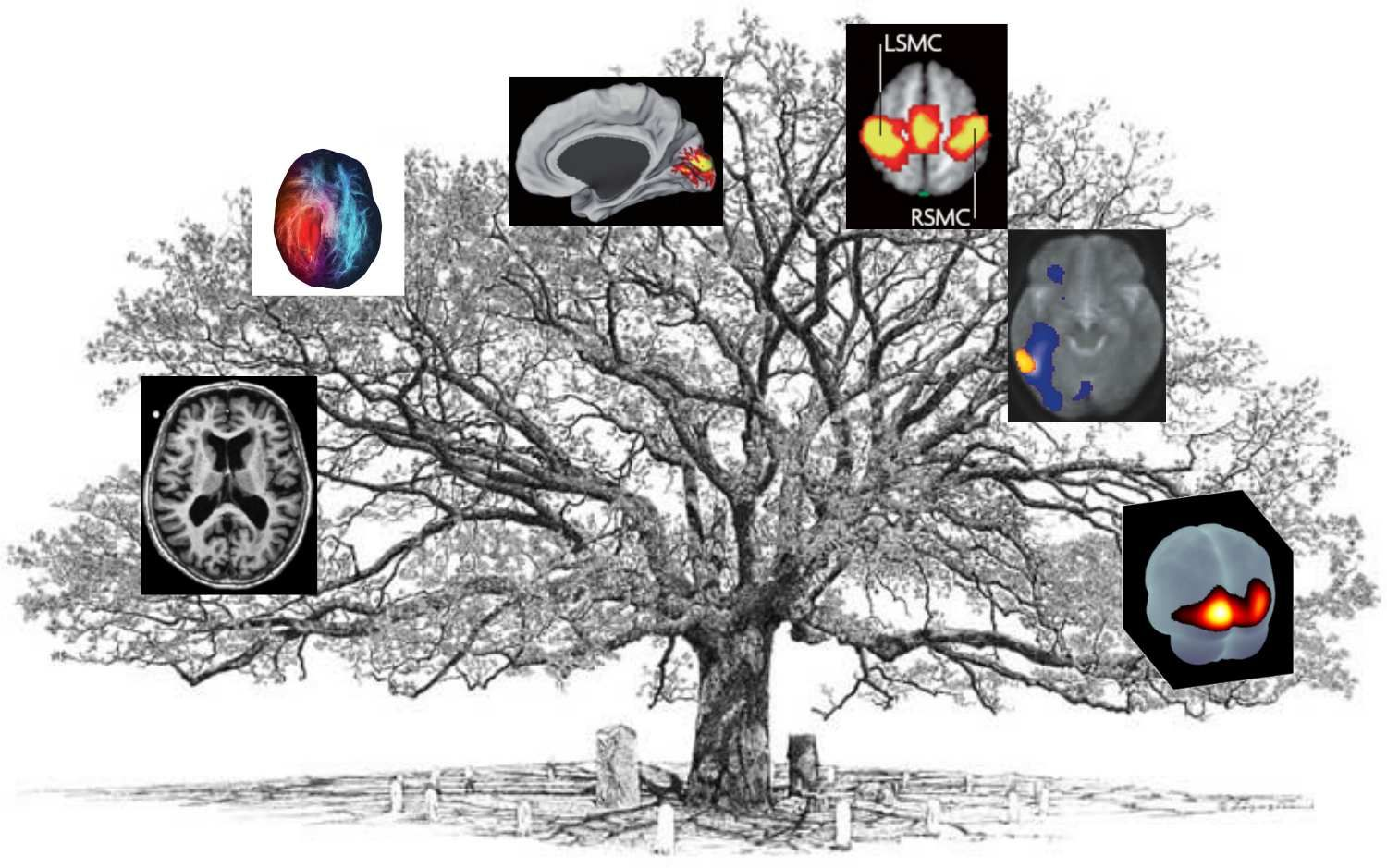
Fig. 1 The neuroimaging tree. Each branch represents one of the techniques that will be briefly presented during this part of the course. Figure adapted by P. Bellec from a variety of non-copyright sources and inspired by the book [Wager and Lindquist, 2015].

This first chapter aims to give an overview of this part of the course as a whole. This is a condensed format, which covers all the imaging techniques that we will briefly discuss during this part of the course. If you want to start your project by studying only one chapter, you’ve come to the right place. But this strategy is not recommended! If, on the contrary, you wish to work on the material of each chapter in depth, the essential information can be found elsewhere in the course notes with more details. Nevertheless, this chapter specifies elements of vocabulary, basic notions and will allow you to quickly make connections between the different techniques seen in this part of the course and beyond.

Objectives 📍

All of the neuroimaging techniques that we will see have distinct strengths and weaknesses, which make them better suited to different types of application. The general objective of this part of the course is for you to understand if a technique is well suited to a research question. For each technique, we aim more specifically to understand four aspects:

• What is the physical principle that allows us to obtain a measurement?

• What is the physiological principle, ie what biological aspect of the brain do we measure?

• What methods of analysis are needed to be able to interpret the data?

• What research questions can be investigated with these techniques?

Structural and functional imaging

Fig. 2 Illustration of the structural and functional techniques briefly discussed in this part of the course, as well as some possible applications in cognitive neuroscience. Figure adapted by P. Bellec from a variety of non-copyright sources and inspired by the book[Wager and Lindquist, 2015].

The techniques studied in this part of the course have in common that they aim to generate maps of the brain. They are also central tools in many cognitive neuroscience studies that use neuroimaging. These techniques include: *Structural Magnetic Resonance Imaging (MRI). This is the best known technique in MRI. It is an image that captures the shape of the brain. It also allows you to see different types of tissue, and in particular the gray matter, that entails the bodies of neurons that are in the brain.

• Diffusion MRI (dMRI). This is another type of image that can be acquired with the same MRI machine as structural MRI. This technique makes it possible to reconstruct the large fiber bundles, i.e. the connections between neurons.

• Functional MRI (fMRI) is yet another type of MRI, specifically used to capture and investigate brain activity. There are two main analysis techniques in fMRI. First, activation maps can be generated when the participant performs a task in the MRI. We will thus look for the regions that are engaged when the participant performs this task. Second, analyzes can also be performed when the participants are in a resting state. With that, we will look at the consistency of activity between different regions. These are functional connectivity cards.

• Positron Emission Tomography (PET) is a technique that does not use MRI (finally!). This technique relies on radioactive tracers that generate gamma rays and cameras that detect these gamma rays. Certain tracers, such as FDG, make it possible to measure cerebral metabolism in relation to the activity of neurons.

• Optical imaging measures changes in the color of blood in the brain, and therefore in its level of oxygenation, which is itself linked to the activity of neurons.

The first two techniques, structural and diffusion MRI, make it possible to study the structure of the brain. The last three techniques (fMRI, PET FDG and optical imaging) all measure functional phenomena. Note that, like MRI, PET can also be used to generate maps of brain structure.

Spatial and temporal resolution

Fig. 3 Illustration of the trade-off between temporal and spatial resolution for the neuroimaging techniques briefly discussed in this part of the course. Figure adapted from

The techniques seen in this part of the course have in common to have a good spatial resolution, but there are nevertheless significant variations between each of these techniques:

• The best from this point of view is the structural MRI whose spatial resolution is excellent, with voxels of approximately 1 mm\(^3\), that is a cube of 1 mm x 1 mm x 1 mm. This allows the structure of the brain to be seen in great detail.

• The dMRI is a little worse, with a spatial resolution closer to 2 mm x 2 mm x 2 mm (8 mm\(^3\)).

• fMRI, on the other hand, commonly uses a resolution of 3 mm x 3 mm x 3 mm - or 27 mm\(^3\), which is almost 30 times larger than the voxel of the structural MRI!

• Finally, PET and optical imaging have a coarser spatial resolution, rather equivalent to 1 cm x 1 cm x 1 cm (i.e. 1000 mm\(^3\)!!). Even if the PET voxels are smaller than 1 cm\(^3\), the image is “blurred” and it is not possible to distinguish small structures.

More on spatial resolution

The notion of spatial resolution generally refers to the minimum size of an object that can be distinguished in an image. If small objects can be distinguished, the resolution is high. If you can only see large objects, the resolution is low. If we are talking about digital photography, the smallest possible object is a pixel, or one of the small squares that make up the image. For maps of the brain, we speak of a voxel, or 3D volume element.

Spatial resolution is not simply the size of a pixel. Two images with the same pixel (or voxel) size can have a different effective resolution if one of the two images is blurry. On the sharp image, smaller objects can be seen than on the blurred image. The effective resolution of the sharp image is therefore higher than that of the blurred image.

Regarding spatial resolution, structural MRI may appear to be the best technique, but there are many other factors to consider when comparing neuroimaging techniques. Another important factor is the temporal resolution. Structural modalities capture changes that are slow to take place. The shape of the cortex and the fiber bundles fall into place throughout development and aging, and they are quite stable even on the scale of several years. In contrast, functional MRI, PET (using FDG), and optical imaging examine brain activity. They measure changes that can occur on the scale of minutes, seconds or even milliseconds.

Temporal resolution

The notion of temporal resolution generally refers to the minimum duration of an event that can be distinguished in a temporal signal. The signals that we see in the course are composed of measurements repeated over time with an interval \(\Delta_t\), generally measured in seconds. We sometimes talk about the sampling frequency, \(f=1/\Delta_t\), measured in Hz. The sampling frequency (Hz) represents the number of measurement points per second.

The temporal resolution does not simply correspond to the time that elapses between two successive measurements \(\Delta_t\). This concept is more difficult to visualize than effective spatial resolution, but is important especially in the case of optical imaging. Optical imaging captures a slow vascular phenomenon. So even if we have peaks of activity separated in time at the neuronal level, if the time interval between the peaks is too short we will only see a single event at the vascular level. It is the equivalent of a blurred image, but in the temporal dimension.

Magnetic resonance imaging

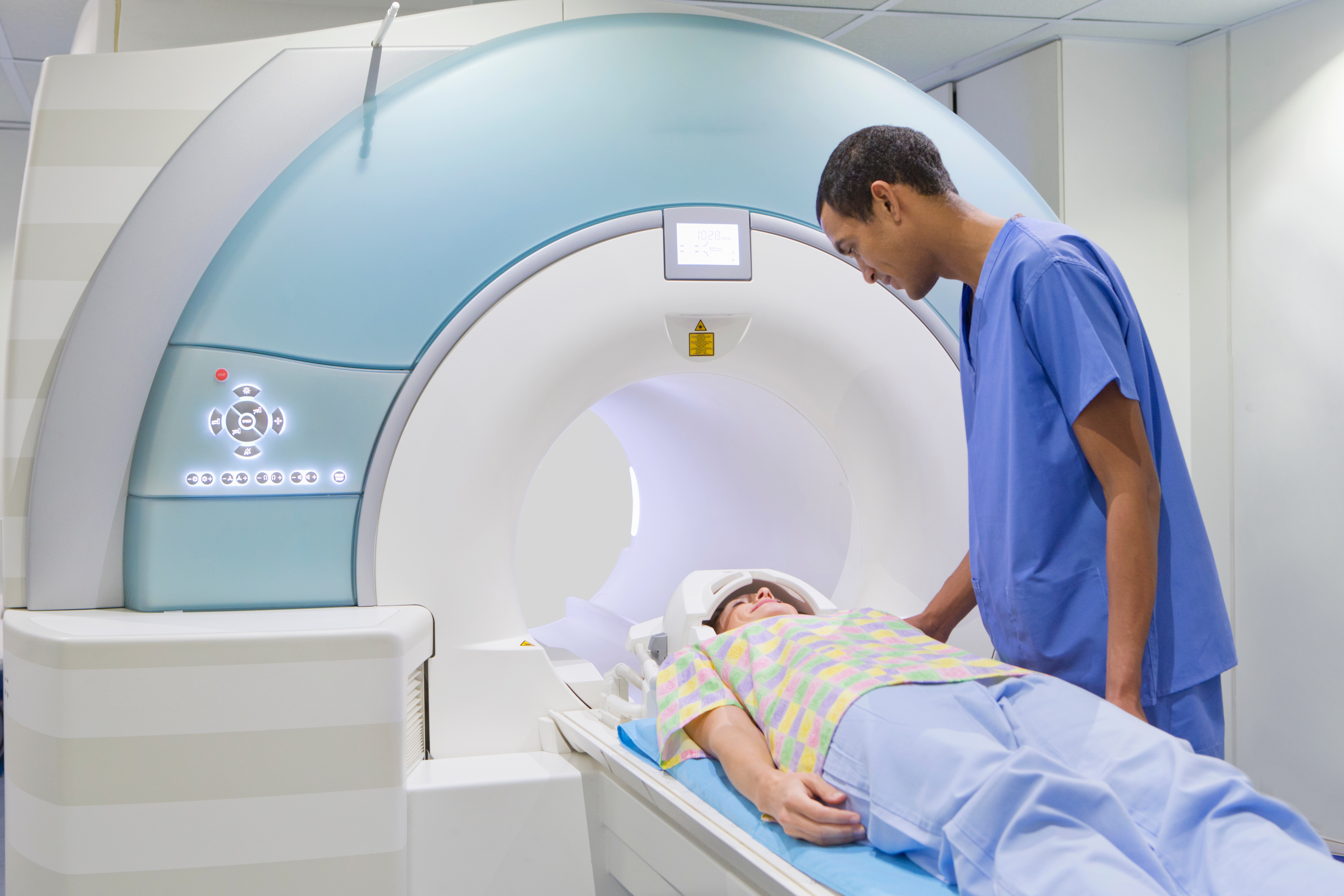
Fig. 4 A functional magnetic resonance imaging machine. Image shutterstock ID 1866109303.

An MRI machine is an imposing machine that can weigh several tens of tons! The most obvious element in an MRI system is the relatively deep tunnel, which is a giant magnet. The participant is positioned on a table which can move to bring the participant to the center of the magnet. The reason for placing the research participant there is that the magnetic field in the center of the magnet is very homogeneous and points in a constant direction. This homogeneous magnetic field, called B0, is like a blank canvas for a painting. Smaller magnets, called gradients, will be turned on and then off quickly to modify the magnetic field in different parts of the brain. As different biological tissues react differently to these stimuli, the gradients allow us to “paint” a picture of the brain on the “canvas” B0. We actually acquire a series of images that will form a 3D volume covering the entire brain. We will discuss the physical process of generating an MRI image in more detail in chapter Functional MRI.

Structural MRI

%matplotlib inline

# This code retrieves T1 MRI data
# and generates an image in three planes of cuts

# ignore warnings
import warnings
warnings.filterwarnings("ignore")

# Download an anatomical scan (here the MNI152 template)
from nilearn.datasets import fetch_icbm152_2009
mni = fetch_icbm152_2009()

# Visualize the 3D brain volume
import matplotlib.pyplot as plt
from myst_nb import glue
from nilearn.plotting import plot_anat, view_img 

t1_fig = plt.figure(figsize=(12, 4))
plot_anat(
  mni.t1,
  axes=t1_fig.gca(),
  black_bg=False,
  dim=0,
  cut_coords=[-17, 0, 17],
  title='T1 weighted MRI',
  output_file='../../../static/neuroscience/mri_example.png'    
)

t1_fig_int = view_img(
  mni.t1,
  cmap='bone',
  colorbar=False,
  bg_img=False,
  dim=-2,
  symmetric_cmap=False,
  title='T1 weighted MRI'
)

glue("t1_fig_int", t1_fig_int, display=False)

interactive

Fig. 5 An example of structural MRI (here with a so-called T1 contrast), on three slice planes: coronal (left), sagital (middle) and axial (right). See the tip {ref} Navigating Through Brain Slices<slices-tip> for an explanation of these terms. This figure is generated by python code using the nilearn library from a public dataset called template MNI152 2009 [Fonov et al., 2011] (click on the + to see the code).

static

Fig. 6 An example of structural MRI (here with a so-called T1 contrast), on three slice planes: coronal (left), sagital (middle) and axial (right). See the tip {ref} Navigating Through Brain Slices<slices-tip> for an explanation of these terms. This figure is generated by python code using the nilearn library from a public dataset called template MNI152 2009 [Fonov et al., 2011] (click on the + to see the code).

The most common type of image acquired with an MRI machine aims to characterize the morphology of the brain. As we can see in the figure above, we easily distinguish some anatomical elements:

• The grey matter, in the periphery of the cortex, appears in gray in the image. This is where the neuron bodies are present.

• It is also possible to distinguish the white matter in white (or rather light gray) which contains bundles of axons - ie the connections between neurons.

• Finally, in black, we can see structures like the ventricles, which contain water, nutrients, as well as metabolic waste.

The size and shape of these structures can vary depending on many behavioral or demographic factors. For example, the amount of gray matter decreases massively with age: this is known as cortical atrophy. Several image analysis techniques have been developed to quantify these morphological changes, such as volumetry, “voxel-based morphometry”, or even surface analyses. These techniques will be presented in the chapter morphometry-chapter.

Navigating through brain slices

There are three main axes used in order to slice the brain: coronal (C), sagital (S), and axial (A), as shown in the figure. In addition, certain terms are commonly used to find their way around these cuts:

• the l (or x) axis typically goes from left to right. When something is near the middle of the brain, it is called a "medial" structure.

• the m (or y) axis goes from the back of the skull (posterior) to the face (anterior). With reference to the mouse, anterior is sometimes called "rostral" (towards the muzzle) and posterior is sometimes called "caudal" (towards the tail).

• the d (or z) axis goes from the feet to the head. The direction of the feet is called "ventral" and the direction of the head is called "dorsal". This terminology makes sense when thinking of a mouse and illogical for humans - but we use it anyway!

Functional MRI

Fig. 7 fMRI data consists of a series of brain volumes. Each voxel is associated with a time series. Figure taken from Nilearn documentation under a BSD license.

Functional MRI is a 4D imaging modality. That is to say that instead of acquiring a single cerebral volume, we acquire a series of them, separated by a time interval called repetition time (TR) (also called \(\Delta_t\) in the {ref} note on temporal resolution <temporal-resolution-tip>). The TR varies from a few hundred milliseconds (uncommon) up to 2 or 3 seconds. The number of repetitions is typically from a few tens to a few hundreds. For each voxel, we therefore have a series of measurement points, which can be represented as a time series. To be able to obtain brain volumes so quickly, one must use large voxels, which range from 2x2x2 mm\(^3\) (uncommon) up to 3x3x3 mm\(^3\) (more standard). With this resolution, we have about 50k voxels in the gray matter (more than 100k when the resolution is close to 2x2x2 mm\(^3\)).

# This code retrieves data from fMRI
# and generates an image of a volume in three section planes

# ignore warnings
import warnings
warnings.filterwarnings("ignore")

# Download a functional scan (ADHD200)
from nilearn.datasets import fetch_adhd
adhd = fetch_adhd(n_subjects=1)

# Visualize one of the 4D volumes
from nilearn.plotting import view_img, plot_img
from nilearn.image import index_img
from myst_nb import glue

func_fig = plt.figure(figsize=(12, 4))
plot_img(index_img(adhd.func[0], 0),
              bg_img=None,
              axes=func_fig.gca(),
              cut_coords=(36, -27, 66),
              black_bg=False,
              title='An fMRI volume',
              output_file='../../../static/neuroscience/fmri_example.png'
)


func_fig_int = view_img(index_img(adhd.func[0], 0),
              bg_img=None,
              cut_coords=(36, -27, 66),
              black_bg=False, cmap='magma',
              title="An fMRI volume")

glue("func_fig_int", func_fig_int, display=False)

interactive

Fig. 8 Example of a single volume in an fMRI series. The volume is represented on three planes of cuts: coronal (left), sagital (middle) and axial (right). See the tip {ref} Navigating Through Brain Slices<slices-tip> for an explanation of these terms. Note that the resolution of the volume is much lower than for anatomical MRI, and it is very difficult to see the details of the anatomy of the brain. This figure is generated by python code using the nilearn library from a public dataset called ADHD200 [Bellec et al., 2017, Milham et al., 2012] (click on the + to see the code).

static

Fig. 9 Example of a single volume in an fMRI series. The volume is represented on three planes of cuts: coronal (left), sagital (middle) and axial (right). See the tip {ref} Navigating Through Brain Slices<slices-tip> for an explanation of these terms. Note that the resolution of the volume is much lower than for anatomical MRI, and it is very difficult to see the details of the anatomy of the brain. This figure is generated by python code using the nilearn library from a public dataset called ADHD200 [Bellec et al., 2017, Milham et al., 2012] (click on the + to see the code).

These measurements do not directly reflect the activity of the neurons, but rather the oxygenation of the blood. We speak of a signal depending on the level of oxygenation in the blood, or BOLD signal (for Blood Oxygen Level Dependent). As we will see in the coupling-neurovascular-section section, this BOLD signal nevertheless indirectly reflects the activity of neurons and will allow us to make maps of brain activity. There are two major types of analysis techniques in fMRI:

• the activation cards: with this approach, we will make the research participant perform certain tasks. For each voxel in the brain, we will then look at whether the level of BOLD activity is higher during a certain task of interest than during a control task. We will talk about this type of analysis technique in chapter Functional MRI.

• connectivity maps: with this approach, the research participant is generally asked to remain at rest, without doing any particular task. We will then examine to what extent the spontaneous activity of different regions of the brain is similar, or synchronous. A high level of synchrony suggests that these regions are engaged in a similar spontaneous cognitive process and therefore form a functional network. We will talk about this type of analysis technique in the chapter Functional connectivity.

Neurovascular coupling

Fig. 10 Realistic 3D rendering of the cerebral vasculature. Picture shutterstock ID 1571296897.

The brain represents only 2% of the body mass, but consumes 20% of the oxygen! The brain therefore needs a regular and large supply of fresh blood which is finely regulated, both spatially (which regions receive a lot of blood) and temporally (the influx of fresh blood changes over time) . The local concentration of oxygenated blood varies according to the local level of activity of the populations of neurons. It is thanks to this mechanism of neurovascular coupling that we can measure the activity of the brain indirectly by means of the vascularization. fMRI is based on this coupling phenomenon as well as optical imaging or PET by FDG. All of these techniques are primarily vascular imaging techniques and are only indirectly related to neuronal activity. Neurovascular coupling is presented in more detail in chapter Functional MRI.

Diffusion MRI

Fig. 11 On the left, a post-mortem brain slice prepared to highlight the white matter fiber bundles. On the right, a virtual dissection of white matter bundles generated using diffusion MRI data. Picture shutterstock ID 412065940.

Diffusion MRI is yet another variety of image that can be acquired, again using an MRI machine. This time, the way of exciting the local magnetic field is specially designed to be sensitive to how water molecules diffuse through a voxel. This type of measurement is repeated many times with different directions and it is thus possible to determine in which direction the water molecules mainly diffuse. This information tells us indirectly about the micro-structure of white matter, because the bundles of fibers made up of axons connecting the neurons to each other come to constrain the way in which water is diffused. Using sophisticated modeling techniques, it is possible to reconstruct in 3D the geometry of the main white matter fibers and to quantify their integrity using different metrics. These metrics can then be associated with different behavioral, demographic or clinical measures, such as, for example, a history of head trauma. This imaging technique will be presented in more detail in the chapter diffusion-mri-chapter.

Optical imaging

Fig. 12 Schematic illustration of the path of near infrared light through the cranium and the brain. Image by Dr Julien Cohen-Adad and Dr Claudine Gauthier.

Optical imaging is our first technique that does not use MRI! But the physiological phenomenon captured by optical imaging is identical to that which is at the origin of the BOLD signal in fMRI. Specifically, this refers to neurovascular coupling. This phenomenon makes it possible to exploit the fact that the concentration of oxygenated hemoglobin indirectly reflects neuronal activity. The big difference between optical imaging and fMRI is how vascular changes are measured. Optical imaging, also sometimes called near-infrared spectroscopy (or near-infrared spectroscopy (NIRS)), uses the fact that near-infrared light can pass through the cranium as well as superficial brain tissue. By a diffusion phenomenon, the light sent directly into the cranial box will come out not far from the source. By analyzing the spectral content, or in other words the color, of the light which has passed through the brain, one can deduce the local concentration of oxygenated and de-oxygenated hemoglobin. These two molecules have indeed different colors and absorb near infrared light very differently. The spatial resolution of optical imaging is much more limited than that of fMRI because the measurements are made at the level of the scalp, as in EEG, rather than thanks to a whole brain image with cubic voxels of controlled size. On the other hand, it is possible to take measurements on the scale of milliseconds. It is important to remember despite everything that the temporal phenomenon studied remains the neurovascular coupling and that this phenomenon is slow (see the warning concerning the effective temporal resolution). This imaging technique will be presented in more detail in the chapter {ref} optical-imaging-chapter.

Positron emission tomography

Fig. 13 Montage of axial sections from a PET scanner with an FDG radiotracer, illustrating the level of glucose metabolic activity over the duration of the scan. Image shutterstock ID 1342194254.

The last neuroimaging modality that this part of the course presents is PET. The functioning of the PET scan is based on the injection of a radioactive product, called a radiotracer, into the blood of the research participant. It may sound scary, but don’t worry. The radioactive dose to which the participant is exposed is low and harmless if the examination is not repeated too often. The radiotracer will accumulate in certain tissues of the brain and emit gamma rays. Gamma rays are actually a very high energy form of light (photons). It is possible to precisely detect the origin of these gamma rays using a series of cameras arranged around the head of the participant and then reconstruct a map of the brain which reflects the concentration of radiotracer at each voxel. The radiotracer to which we will mainly refer during this course is fluorodeoxyglucose (FDG). This is consumed as fuel indirectly by the neurons, just like oxygen. FDG PET therefore works through neurovascular coupling, just like fMRI and optical imaging. On the other hand, it takes several minutes to build a map of brain activity, so the temporal resolution of PET is lower than that of fMRI and PET. Furthermore, as you can observe on the images above, the reconstructed PET maps are blurred and the effective spatial resolution of the images is less than the size of the voxels. Finally, it is important to know that many other tracers exist apart from FDG. In particular, there are structural tracers. Like MRI, PET can therefore be used to generate structural and functional images of the brain. This imaging technique will be presented in more detail in chapter PET-chapter.

Statistical maps

# Import visualization libraries
# and prepare the layout of the figure
import numpy as np
import matplotlib.pyplot as plt
fig = plt.figure(figsize=(12, 4))

# ignore warnings
import warnings
warnings.filterwarnings("ignore")

# Download a motor activation contrast from NeuroVault
from nilearn import datasets
motor_images = datasets.fetch_neurovault_motor_task()
stat_img = motor_images.images[0]

# Visualization of the 3D brain volume
from nilearn.plotting import plot_stat_map
from myst_nb import glue


stat_map_fig = plt.figure(figsize=(12, 4))
plot_stat_map(stat_img,
              axes=stat_map_fig.gca(),
              cut_coords=(36, -27, 66),
              black_bg=False,
              title='Statistical map related to movements',
              output_file='../../../static/neuroscience/stat_map_example.png'
)


stat_map_fig_int = view_img(stat_img,
                   threshold=3,
                   title="Statistical map related to movements",
                   cut_coords=[36, -27, 66], cmap='RdBu_r'
                   )

glue("stat_map_fig_int", stat_map_fig_int, display=False)

<Figure size 864x288 with 0 Axes>

interactive

Fig. 14 A regression model is applied to each voxel to generate a statistical brain map. Here, the statistical map corresponds to changes in fMRI activation during hand movements. The statistical map is visualized thanks to this nilearn tutorial and a motor activity map distributed via NeuroVault. Click on the + to see the code.

static

Fig. 15 A regression model is applied to each voxel to generate a statistical brain map. Here, the statistical map corresponds to changes in fMRI activation during hand movements. The statistical map is visualized thanks to this nilearn tutorial and a motor activity map distributed via NeuroVault. Click on the + to see the code.

The last important aspect that will be covered in these lecture notes is a discussion of how to analyze data. This notably involves the image analysis steps that are necessary to generate interpretable measurements. This also involves making statistics on the images of the brain that are generated. There are many ways to perform these statistical analyzes and the field of cognitive neuroscience is increasingly using multivariate machine learning techniques. But the reference technique remains the linear regression model which is applied independently to each voxel, also called mass-univariate statistics. This is a very flexible model that can answer a large number of questions, both at individual and group level. The linear regression model is used by all the neuroimaging techniques seen during this part of the course. The fact of repeating a statistical test at each voxel, tens of thousands of times, also poses a problem when the time comes to establish the significance threshold. We will discuss linear regression and thresholding approaches in chapter maps-statistics-chapter. Finally, it is possible to abuse this type of statistical model in many ways and thus lead to the publication of non-reproducible results. We will discuss these challenges and possible solutions in the final chapter: reproducibility-controversies-chapter.

Conclusions

This chapter has given you a quick overview of the different methods used in cognitive neuroscience that will be presented in this part of the course. We hope this inspires you to learn more and explore these lecture notes!

References

1(1,2)

Pierre Bellec, Carlton Chu, François Chouinard-Decorte, Yassine Benhajali, Daniel S. Margulies, and R. Cameron Craddock. The Neuro Bureau ADHD-200 Preprocessed repository. NeuroImage, 144:275–286, January 2017. URL: https://www.sciencedirect.com/science/article/pii/S105381191630283X (visited on 2022-04-01), doi:10.1016/j.neuroimage.2016.06.034.

2(1,2)

Vladimir Fonov, Alan C. Evans, Kelly Botteron, C. Robert Almli, Robert C. McKinstry, and D. Louis Collins. Unbiased average age-appropriate atlases for pediatric studies. NeuroImage, 54(1):313–327, January 2011. URL: https://www.sciencedirect.com/science/article/pii/S1053811910010062 (visited on 2022-04-01), doi:10.1016/j.neuroimage.2010.07.033.

3(1,2)

Michael Milham, Damien Fair, Maarten Mennes, and Stewart Mostofsky. The adhd-200 consortium: a model to advance the translational potential of neuroimaging in clinical neuroscience. Frontiers in Systems Neuroscience, 2012. URL: https://www.frontiersin.org/article/10.3389/fnsys.2012.00062 (visited on 2022-04-01).

4(1,2)

Tor D. Wager and Martin A. Lindquist. Principles of fMRI. Leanpub, July 2015. URL: https://leanpub.com/principlesoffmri (visited on 2022-04-19).

Exercises

In the following we created a few exercises that aim to recap core aspects of this part of the course and thus should allow you to assess if you understood the main points.

Exercise 1.1

We perform a visual stimulation for 100 ms and we want to study the cerebral response in the occipital cortex.

• Name a strength and a weakness of fMRI and EEG to study this question.

• Explain why.

Exercise 1.2

Rank these techniques according to their spatial resolution (starting with the most precise):

1. fMRI

2. structural MRI

3. PET

Exercise 1.3

Rank these techniques according to their temporal resolution (starting with the most precise):

1. fMRI

2. Optical Imaging

3. EEG

4. Diffusion MRI

Exercise 1.4

An activation of the ipsilateral motor cortex is observed in the context of a movement of the right hand, following a stroke. This observation is made using fMRI.

1. Name a possible limitation of this observation, in the specific context of this experiment.

2. Propose an additional experience allowing to answer this limitation, and describe what it brings as a complement.

Exercise 1.5

One study participant suffered from an accident that left metallic debris in his eye in the past.

1. Name an imaging technique for which it is a contraindication. Explain why.

2. Name a technique for which this is not a problem. Explain why.

Exercise 1.6

We wish to measure the response of the motor cortex to motor activation longitudinally in a participant. More specifically, a functional imaging acquisition is performed every two weeks for three months.

• In the specific context of this experience, name a problem and a strength of the F18-FDG PET.

Exercise 1.7

To answer this question, read the article by Shukla et al, “Aberrant Frontostriatal Connectivity in Negative Symptoms of Schizophrenia”, published in Schizophrenia Bulletin (2019, 45(5): 1051-59) and available open access at this address. The following questions are short answers.

• What type(s) of participant(s) were recruited into this study?

• What is the main objective of the study?

• What are the inclusion and exclusion criteria?

• Which neuroimaging technique(s) is(are) used? Is it a structural or functional technique?

• Where are the regions of interest used in the study described? How are they defined?

• Where are the imaging parameters used in the study described? List parameters used.

• Which figure meets the main objective of the study? What is the main conclusion?

Exercise 1.8

We want to compare different aspects of cerebral architecture between a population of schizophrenic patients and a population of control participants.

• We are interested in the cerebral processing of visual stimuli composed of images with a strong emotional valence. What imaging modality and analysis technique would you use and why?

• We are interested in a possible atrophy of the frontal cortex. What imaging modality and analysis technique would you use and why?

• We want to study spontaneous brain activity and acquire as large a sample as possible with a fixed budget. What imaging modality and analysis technique would you use and why?

previous

Introduction II - Neuroscience

next

Magnetic Resonance Imaging (MRI)