Diffusion MRI¶

../../../_images/fig_dissection_virtuelle.jpg

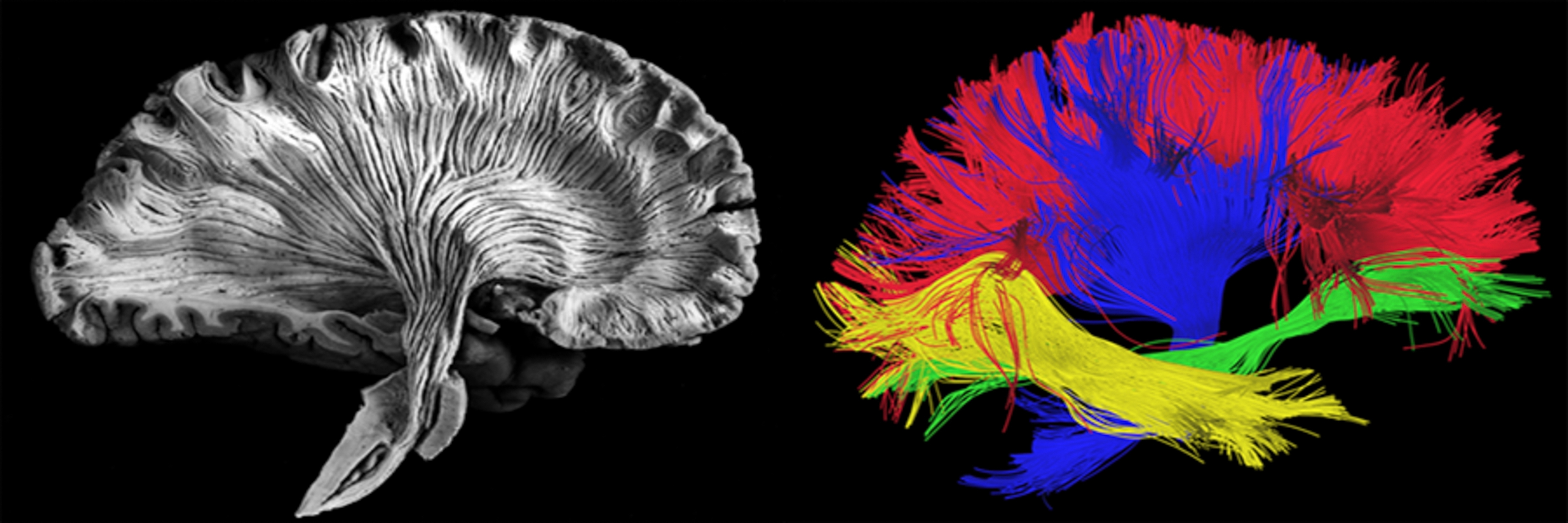
Fig. 44 On the left, a post-mortem brain slice prepared to highlight the white matter fiber bundles. On the right, a virtual dissection of white matter bundles generated using diffusion MRI data. Picture shutterstock ID 412065940.¶

Objectives¶

The purpose of this part of the course is to introduce you to the principles of diffusion magnetic resonance imaging (dMRI). dMRI is a neuroimaging modality that allows us to study white matter fibres. We are therefore able to examine the connections between different regions, both interhemispheric (i.e., white matter fibers traveling from one hemisphere to another), and intrahemispheric (i.e., white matter fibers traveling within the same hemisphere) . To get a concrete idea of what white matter fibers look like, you can watch this video presenting brain dissections, taken from the course of Functional Neuroanatomy from UBC.

from IPython.display import HTML
import warnings
warnings.filterwarnings("ignore")

# Youtube
HTML('<iframe width="560" height="315" src="https://www.youtube.com/embed/PazaHElk6wc" title="YouTube video player" frameborder="0" allow="accelerometer; autoplay; clipboard-write; encrypted-media; gyroscope; picture-in-picture" allowfullscreen></iframe>')

During this lesson, we will cover:

The physical and physiological principles of the signal in dMRI.
The model of the diffusion tensor.
tractography analyses.

Physical and physiological principles¶

Water diffusion¶

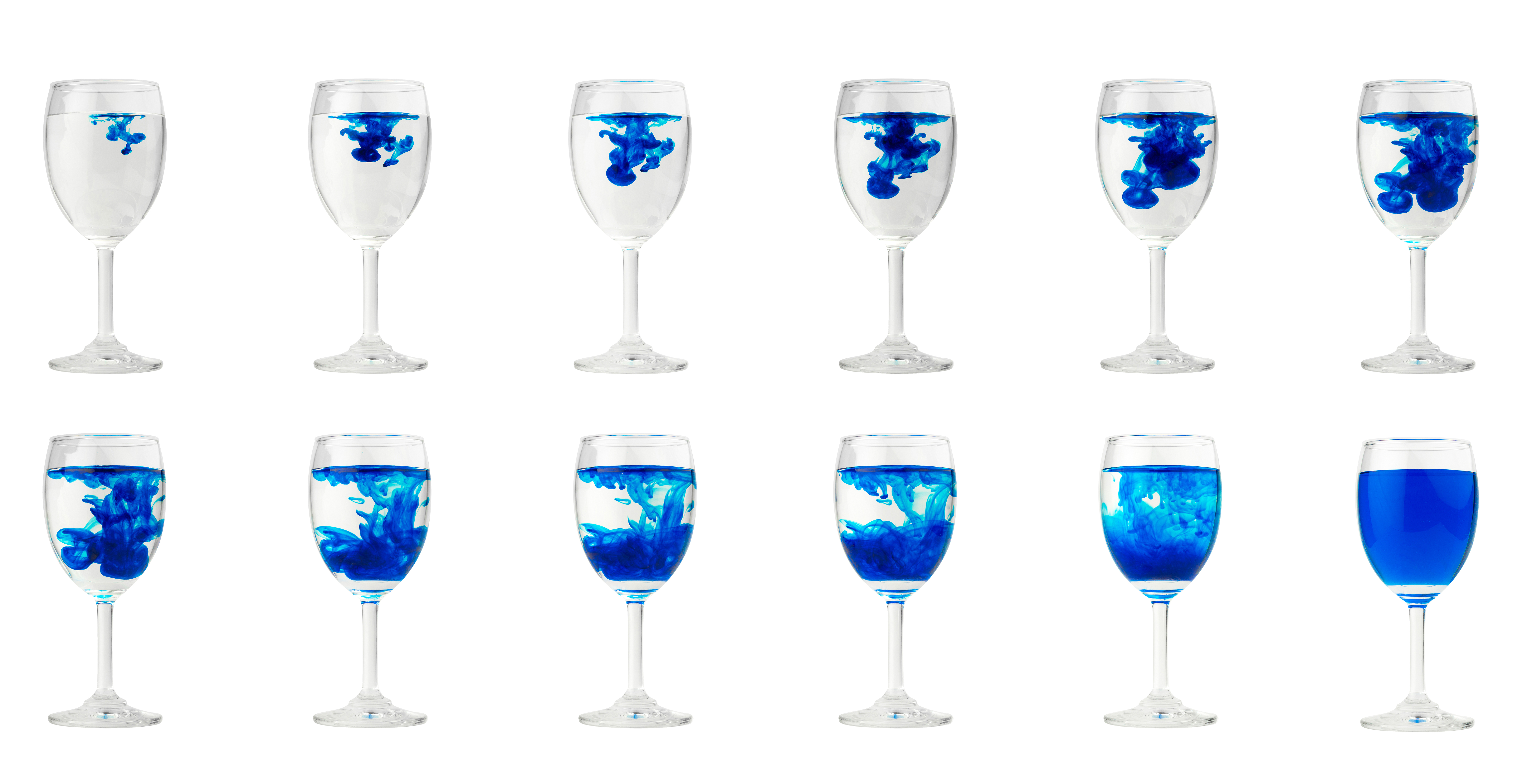
Fig. 45 Illustration of the diffusion of a drop of ink in a glass of water. Image by Narudon Atsawalarpsakun available at [shutterstock](https://www.shutterstock.com/image-photo/blue-food-coloring-diffuse -water-inside-736860766) ID 736860766, used under standard shutterstock license.¶

In diffusion MRI, we are interested in the way water diffuses in the brain. By examining how water diffuses, we can learn information about the medium of diffusion, in our case, the brain! Specifically, dMRI allows us to learn more about the microstructure properties of white matter fibers. For a concrete example of diffusion, we can imagine what happens when we drop a drop of ink into a glass of water, illustrated as Fig. 45. The ink will over time diffuse into the water, coloring the water little by little, until it becomes homogeneously colored. Water and ink molecules collide in random directions, and follow a random walk process called Brownian motion, see brownian-fig.

"""Brownian motion
code adapted from Scipy Cookbook https://scipy-cookbook.readthedocs.io/items/BrownianMotion.html
under an MIT-like license https://github.com/scipy/scipy-cookbook/blob/master/LICENSE.txt
"""
def brownian(x0, n, dt, delta, out=None):
    """
    Generate an instance of Brownian motion (i.e. the Wiener process):

        X(t) = X(0) + N(0, delta**2 * t; 0, t)

    where N(a,b; t0, t1) is a normally distributed random variable with mean a and
    variance b.  The parameters t0 and t1 make explicit the statistical
    independence of N on different time intervals; that is, if [t0, t1) and
    [t2, t3) are disjoint intervals, then N(a, b; t0, t1) and N(a, b; t2, t3)
    are independent.

    Written as an iteration scheme,

        X(t + dt) = X(t) + N(0, delta**2 * dt; t, t+dt)


    If `x0` is an array (or array-like), each value in `x0` is treated as
    an initial condition, and the value returned is a numpy array with one
    more dimension than `x0`.

    Arguments
    ---------
    x0 : float or numpy array (or something that can be converted to a numpy array
         using numpy.asarray(x0)).
        The initial condition(s) (i.e. position(s)) of the Brownian motion.
    n : int
        The number of steps to take.
    dt : float
        The time step.
    delta : float
        delta determines the "speed" of the Brownian motion.  The random variable
        of the position at time t, X(t), has a normal distribution whose mean is
        the position at time t=0 and whose variance is delta**2*t.
    out : numpy array or None
        If `out` is not None, it specifies the array in which to put the
        result.  If `out` is None, a new numpy array is created and returned.

    Returns
    -------
    A numpy array of floats with shape `x0.shape + (n,)`.

    Note that the initial value `x0` is not included in the returned array.
    """


    x0 = np.asarray(x0)

    # For each element of x0, generate a sample of n numbers from a
    # normal distribution.
    if len(delta)>1:
        r = np.empty(x0.shape + (n,))
        r[0, :] = norm.rvs(size=(n,), scale=delta[0] * sqrt(dt))
        r[1, :] = norm.rvs(size=(n,), scale=delta[1] * sqrt(dt))
        r[2, :] = norm.rvs(size=(n,), scale=delta[2] * sqrt(dt))
    else:
        r = norm.rvs(size=x0.shape + (n,), scale=delta[0] * sqrt(dt))

    # If `out` was not given, create an output array.
    if out is None:
        out = np.empty(r.shape)

    # This computes the Brownian motion by forming the cumulative sum of
    # the random samples.
    np.cumsum(r, axis=-1, out=out)

    # Add the initial condition.
    out += np.expand_dims(x0, axis=-1)

    return out

import numpy as np
from matplotlib import pyplot as plt
from math import sqrt
from scipy.stats import norm

# The Wiener process parameter.
delta = [0.25]
# Total time.
T = 10.0
# Number of steps.
N = 500
# Time step size
dt = T/N
# Initial values of x.
x = np.empty((2,N+1))
x[:, 0] = 0.0

fig = plt.figure(figsize=(5, 5), dpi=100)
ax = plt.axes()
n_samp = 10
points = np.empty((2, n_samp))
for samp in range(n_samp):
    brownian(x[:,0], N, dt, delta, out=x[:,1:])

    # Plot the 2D trajectory.
    ax.plot(x[0, :], x[1, :])
    points[:, samp] = x[:, -1]

# Mark the start and end points.
ax.plot(x[0,0], x[1,0], 'ro', markersize=12, alpha=0.5)
for samp in range(n_samp):
    ax.plot(points[0, samp], points[1, samp],'bo', markersize=12, alpha=0.5)

# More plot decorations.
plt.title('Brownien 2D motion')
ax.set_xlabel('X axis')
ax.set_ylabel('Y axis')
ax.set_xlim([-2.5, 2.5])
ax.set_ylim([-2.5, 2.5])

# Glue the figure
from myst_nb import glue
glue("brownian-fig", fig, display=False)

plt.close()

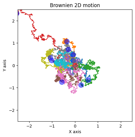
Fig. 46 Illustration of Brownian motion of a molecule. The starting point is indicated by a red circle. The color trajectories correspond to simulated random walks following a Brownian movement. The blue dots indicate the end point of each step. Figure generated using Python code by P. Bellec, licensed under CC-BY 4.0. The Brownian motion simulation code is adapted from Scipy Cookbook under a license close to MIT.¶

Isotropic and anisotropic diffusion¶

list_speed = (0.25, 0.5, 0.75)

# Initial values of x.
x = np.empty((3,N+1))
x[:, 0] = 0.0
fig = plt.figure(figsize=(13, 5), dpi=100)
for num, speed in enumerate(list_speed):
    fig.add_subplot(1, len(list_speed), num + 1, projection='3d')
    ax = plt.gca()
    n_samp = 1000
    delta=np.array([speed, 0.25, 0.25])
    bounds = [8, 8, 8]
    points = np.empty((3, n_samp))
    for samp in range(n_samp):
        brownian(x[:,0], N, dt, delta, out=x[:,1:])
        points[:, samp] = x[:, -1]
    ax.scatter(points[0, :], points[1, :], points[2, :], 'o', alpha=0.2)
    ax.set_box_aspect([ax.get_xlim()[1] - ax.get_xlim()[0],
                       ax.get_ylim()[1] - ax.get_ylim()[0],
                       ax.get_zlim()[1] - ax.get_zlim()[0]]
                    )
    ax.set_title(f'speed x = {speed}')
    ax.set_xlabel('x')
    ax.set_ylabel('y')
    ax.set_zlabel('z')

# Glue the figure
from myst_nb import glue
glue("anisotropic-fig", fig, display=False)  

plt.close()

Fig. 47 Isotropic vs anisotropic diffusion. Each blue circle represents the arrival point of a water molecule according to a random walk simulation with a 3D Brownian process. On the graph on the left, the diffusion rate of water molecules is identical in all directions. On the graphs in the middle and on the right, the diffusion velocity is greater along the x axis than along the y and z axes. Figure generated using Python code by P. Bellec, licensed CC-BY 4.0.¶

The movement of water molecules in a medium follows a Brownian motion. If the medium has similar characteristics in all directions, it is said to be an isotropic medium. The left graph of the Fig. 47 represents the set of endpoints of random walks in such an isotropic medium. We notice that the molecules are distributed approximately in a sphere. What if the diffusion is faster in a given direction, for example the x axis? We then speak of an anisotropic medium. On the middle graph, we see that the shape filled by the molecules is getting longer, and looks more like an American football than a sphere (or, in mathematical terms, an ellipse). The more the diffusion velocity difference on x grows with respect to the y and z directions, the more the shape lengthens (graph on the right).

Diffusion and white matter fibers¶

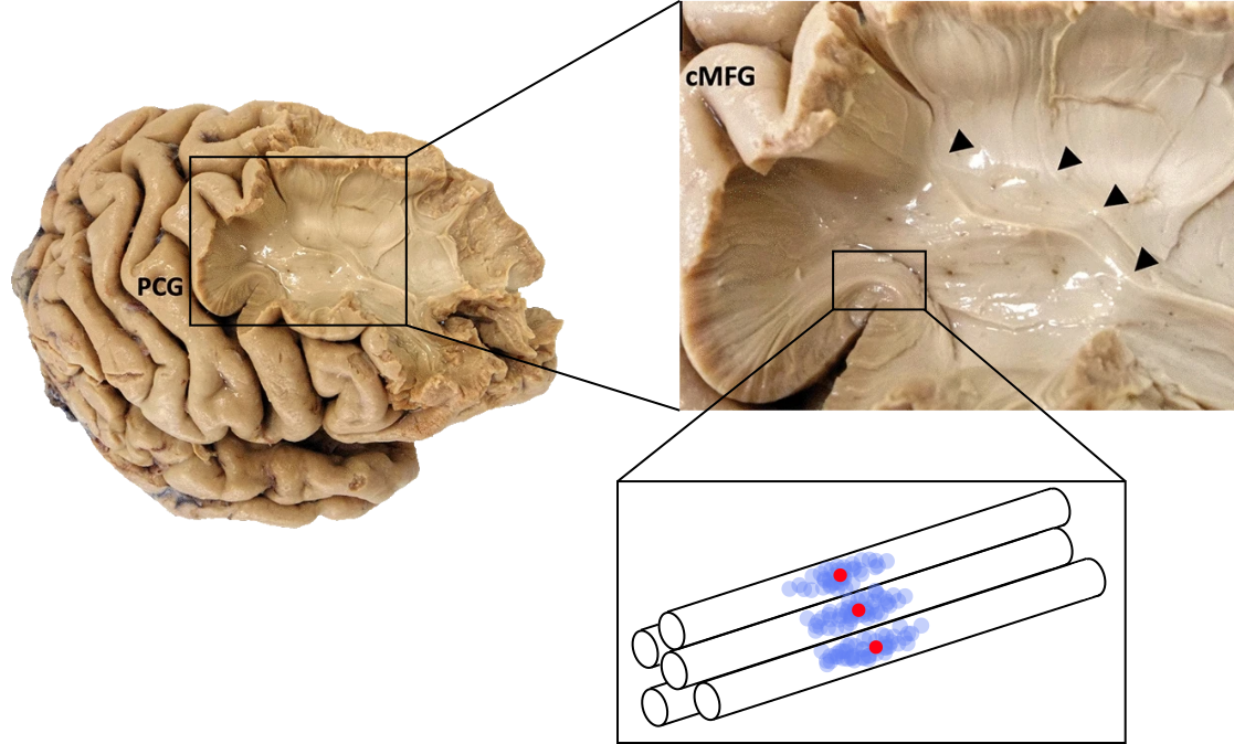
Fig. 48 Cerebral dissection illustrating the organization of cerebral white matter into fiber bundles. Bottom right: diagram illustrating the diffusion of water constrained by the fibres. The red dot corresponds to the origin of random walks, whose terminations are indicated by the blue dots. Brain images taken from [Bakhit et al., 2020], licensed under CC-BY 4.0. The rest of the figure by P Bellec, under license CC-BY 4.0, inspired by the thesis of C. Poupon, 1999.¶

The axons of the neurons come to constrain the diffusion of water, the water molecules can therefore not move freely in all directions. The diffusion profile of the water molecules then follows an anisotropic shape, as we have just seen in Fig. 47. Water diffuses more easily in the direction parallel to the fibres. Diffusion is therefore anisotropic and the diffusion coefficient will then be higher in this parallel direction, see Fig. 48. So by knowing how water diffuses, we can determine the configuration of the axons. The phenomenon of diffusion depends on the structure of the fabric! This is the physiological principle at the origin of dMRI measurements.

dMRI acquisition¶

import numpy as np
from dipy.data import get_fnames
from dipy.io.image import load_nifti, save_nifti
import matplotlib.pyplot as plt

hardi_fname, hardi_bval_fname, hardi_bvec_fname = get_fnames('stanford_hardi')
data, affine = load_nifti(hardi_fname)

sli = data.shape[2] // 2
list_vol = [10, 40, 50]  # pick out random volumes and gradient directions

fig1, ax = plt.subplots(1, 3, figsize=(12, 6),
                        subplot_kw={'xticks': [], 'yticks': []})
fig1.subplots_adjust(hspace=0.3, wspace=0.05)

for num, vol in enumerate(list_vol):
    vol_slice = data[:, :, sli, vol]

    ax.flat[num].imshow(vol_slice.T, cmap='gray', interpolation='none',
                  origin='lower')
    ax.flat[num].set_title(f'direction {num+1}')
# Glue the figure
from myst_nb import glue
glue("diffusion-direction-fig", fig1, display=False)  

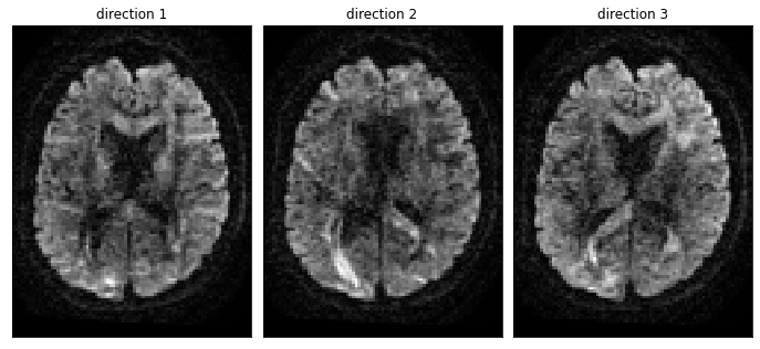
Fig. 49 Diffusion-weighted MRI volumes. Each axial slice represents a diffusion-weighted T2* volume for a different direction. Figure generated using Python code by P. Bellec, licensed CC-BY 4.0. The code is adapted from a tutorial of the DIPY library, distributed under the BSD 3-Clause license.¶

In diffusion MRI, we take images in several orientations. These are T2*-weighted images that we acquire using dMRI data acquisition protocol. The applied sequence makes the image sensitive to water diffusion, in a given direction. For a given voxel, we’ll take measurements in different directions, which will tell us if the water has diffused a lot in that direction, much like the blue dots in the Fig. 48. For a dMRI volume, the value in a voxel tells us if the blue point is far or not from the red point, for a direction that we have selected, see diffusion-direction-fig

Diffusion tensor¶

The tensor model¶

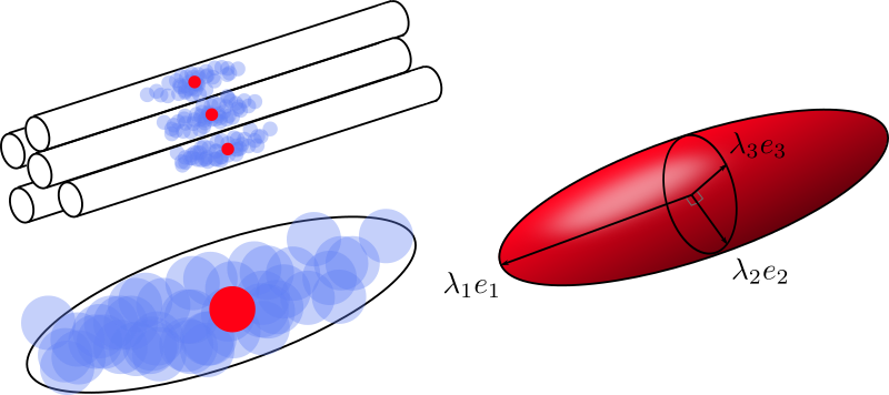
Fig. 50 The diffusion of water molecules over time can be visualized as a cloud of points. Due to the constraints of the environment, in particular the axons, this cloud takes the form of a rugby ball (top, left). The shape of the cloud can be approximated with a tensor model (bottom left). The main parameters of this model are the main diffusion directions \(e_1\), \(e_2\), \(e_3\), as well as the diffusion values associated with these directions \(\lambda_1 \geq \lambda_2 \geq \lambda_3\). Figure by P. Bellec under license CC-BY 4.0, inspired by M. Descoteaux and C. Poupon.¶

From the simulations above, it is intuitive to imagine the diffusion of water as a balloon, more or less elongated. Mathematically, this is formulated with a diffusion tensor, or Gaussian model, see Fig. 50. To estimate the shape of our balloon in each voxel, we use the different scattering values obtained for each acquisition direction. If the spread is greater in a certain direction, our ball will look more like a rugby ball. If the diffusion is similar in all acquisition directions, we will obtain a soccer ball instead.

Diffusion Tensor Imaging¶

# Import modules
import numpy as np
from dipy.io.image import load_nifti, save_nifti
from dipy.io.gradients import read_bvals_bvecs
from dipy.core.gradients import gradient_table
import dipy.reconst.dti as dti
from dipy.data import get_fnames

# Select patch
minx = 1
maxx = 81
miny = 1
maxy = 106
minz = 28
maxz = 32

# Download HARDI data
hardi_fname, hardi_bval_fname, hardi_bvec_fname = get_fnames('stanford_hardi')
data, affine = load_nifti(hardi_fname)
bvals, bvecs = read_bvals_bvecs(hardi_bval_fname, hardi_bvec_fname)
gtab = gradient_table(bvals, bvecs)

# Force affine to something simple to make it easier to extract patches
affine = np.eye(4)

# Mask data and estimate tensors
from dipy.segment.mask import median_otsu
data = data[:, :, minz:maxz, :]
maskdata, mask = median_otsu(data, vol_idx=range(10, 50), median_radius=3,
                             numpass=1, autocrop=True, dilate=2)
tenmodel = dti.TensorModel(gtab)
tenfit = tenmodel.fit(maskdata)

# Generate derived metrics (FA etc)
from dipy.reconst.dti import fractional_anisotropy, color_fa
FA = fractional_anisotropy(tenfit.evals)
FA[np.isnan(FA)] = 0
FA = np.clip(FA, 0, 1)
RGB = color_fa(FA, tenfit.evecs)
MD1 = dti.mean_diffusivity(tenfit.evals)

# Figure
from dipy.data import get_sphere
sphere = get_sphere('repulsion724')
from dipy.viz import window, actor
scene = window.Scene()
evals = tenfit.evals[minx:maxx, miny:maxy, :]
evecs = tenfit.evecs[minx:maxx, miny:maxy, :]

# boost the colors
RGB *= 2
RGB[RGB>1] = 1
cfa = RGB[minx:maxx, miny:maxy, :]
scene.add(actor.tensor_slicer(evals, evecs, scalar_colors=cfa, sphere=sphere,
                              scale=0.3))
scene.set_camera(position=(14.87946710578175, 25.770232149765413, 173.54578028650144),
                 focal_point=(33.43851200470716, 40.67356830562871, 15.545914873824975),
                 view_up=(0.003256400517440014, 0.9955397521536979, 0.09428678453221151))
window.record(scene, n_frames=1, out_path='tensor-slice.png',
              size=(1000, 1000), reset_camera=False)
scene.set_camera(position=(6.398539759431944, 36.122368120824724, 21.074961978614017),
                 focal_point=(17.02336666201742, 55.39317316617157, 7.230217513090364),
                 view_up=(0.10205867972271891, 0.5426923506538308, 0.8337080055001721))
window.record(scene, n_frames=1, out_path='tensor-zoom.png',
              size=(600, 600), reset_camera=False)             

# Make figure
from matplotlib import pyplot as plt
import imageio
fig1, ax = plt.subplots(1, 2, figsize=(12, 6), dpi=200,
                        subplot_kw={'xticks': [], 'yticks': []})
fig1.subplots_adjust(hspace=0.3, wspace=0.05)
im = imageio.imread('tensor-slice.png')
ax.flat[0].imshow(im, interpolation='antialiased')
ax.flat[0].set_title('full slice')
im = imageio.imread('tensor-zoom.png')
ax.flat[1].imshow(im, interpolation='none')
ax.flat[1].set_title('zoom')

# Glue the figure
from myst_nb import glue
glue("tensor-fig", fig1, display=False)

plt.close()

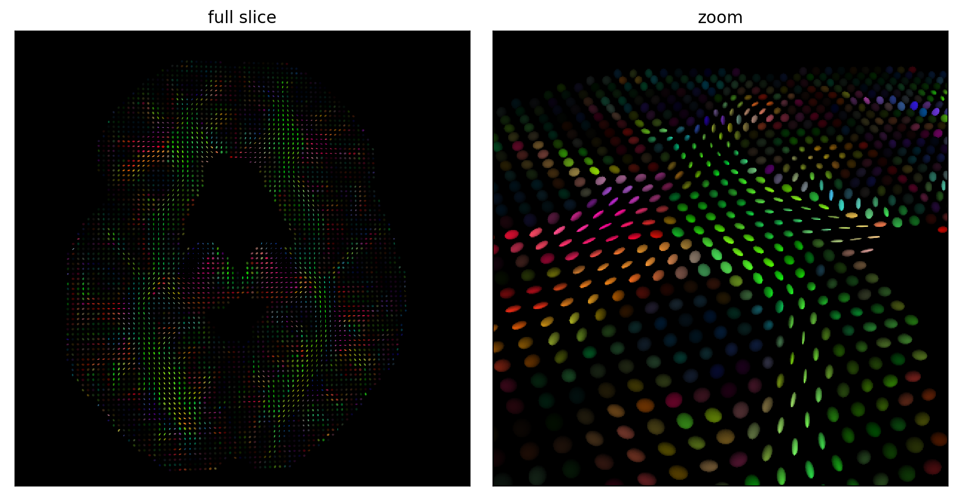
Fig. 51 Diffusion tensors estimated on an axial slice (left) and zoom on a portion of the slice (right). The color of each tensor codes for the main direction of diffusion, as well as the fractional anisotropy of each tensor. The brightest tensors are strongly anisotropic, ie the principal direction of diffusion is clearly stronger than the transverse directions. Figure generated by python code adapted from a DIPY tutorial by P. Bellec under license CC- BY 4.0.¶

Diffusion tensor imaging (diffusion tensor imaging, DTI) is one of the first analysis techniques that emerged in diffusion MRI. To estimate the shape of our balloon, we need at least six acquisition directions: xy, xz, yz, -xy, -xz, y-z. It is by combining the images in these six directions that we can estimate our diffusion tensor (our balloon). Since we have these measurements for each of the voxels, we can create a brain volume where the value of each voxel is a tensor (balloon), see Fig. 51.

Characteristics of tensors¶

import matplotlib.pyplot as plt
RGB2 = np.empty([RGB.shape[1], RGB.shape[0], RGB.shape[3]])
MD = MD1
MD[mask==0] = 0

for num in range(3):
    RGB2[:, :, num] = np.squeeze(RGB[:, :, 0, num]).T

fig1, ax = plt.subplots(1, 3, figsize=(12, 6),
                        subplot_kw={'xticks': [], 'yticks': []})

fig1.subplots_adjust(hspace=0.3, wspace=0.05)
ax.flat[0].imshow(np.squeeze(FA[:, :, 0]).T, origin='lower',
                  cmap='gray', vmin=0, vmax=1)
ax.flat[0].set_title('FA map')
ax.flat[1].imshow(np.squeeze(MD[:, :, 0]).T, origin='lower',
                  cmap='gray')
ax.flat[1].set_title('DM map')
ax.flat[2].imshow(RGB2, origin='lower')
ax.flat[2].set_title('principal direction')

# Glue the figure
from myst_nb import glue
glue("fa-md-rgb-fig", fig1, display=False)

plt.close()

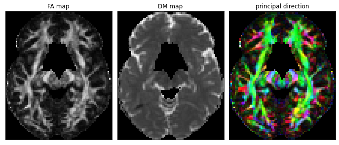
Fig. 52 Tensor-derived maps in diffusion MRI: fractional anisotropy (left), mean diffusivity (middle) and principal direction of the tensor (right). For the main direction, the medial-lateral (x) axis is coded in red, the anterior-posterior (y) axis is coded in green, and the ventral-dorsal (z) axis is coded in blue. Figure generated using Python code adapted from a DIPY tutorial by P. Bellec, under license CC-BY 4.0.¶

It is possible to summarize some important characteristics of diffusion tensors using a single measure, such as fractional anisotropy and mean diffusivity (see definitions below). We therefore extract a measurement per voxel, which can be represented with a cerebral map, in a similar way to what we have seen with T1 or T2 weighted images, see fa-md-rgb- fig. It is also possible to create a color image, which codes for the main direction of diffusion.

Fractional Anisotropy

A popular measure is Fractional Anisotropy (FA), which measures the degree of anisotropy of a diffusion phenomenon, by taking values between 0 and 1. A fractional anisotropy value of 0 indicates isotropic diffusion (soccer ball), while a value of 1 indicates strongly anisotropic diffusion (rugby ball). Note that the fractional anisotropy of water is 0, unless diffusion is constrained by a structure. Strong FA values are usually found in white matter.

Average Diffusivity

We can also measure the mean diffusivity according to the following equation (see Fig. 50 for notations): \(\overline{\lambda} = \frac{\lambda_{1}+\lambda_{2}+\lambda_{3}}{3}\) The average diffusivity tells us how much diffusion there is inside a voxel. The average diffusivity is very strong in the cerebrospinal fluid, where the water molecules are very little constrained.

Main Direction of Dissemination

In order to visualize which main direction the tensors point, a popular approach is to encode each x, y, and z axis with a color (red, green, blue, respectively). For a given direction, the three colors are mixed in a proportion corresponding to the contributions of the three axes.

Tractography¶

Streamline Tractography¶

from matplotlib import pyplot as plt
MD = MD1
MD[mask==0] = 0
threshold_fa = 0.3
mask_wm = FA > threshold_fa


fig1, ax = plt.subplots(1, 2, figsize=(12, 6),
                        subplot_kw={'xticks': [], 'yticks': []})

fig1.subplots_adjust(hspace=0.3, wspace=0.05)
ax.flat[0].imshow(np.squeeze(FA[:, :, 0]).T, origin='lower',
                  cmap='gray', vmin=0, vmax=1)
ax.flat[0].set_title('fractional anisotropy map')
ax.flat[1].imshow(np.squeeze(mask_wm[:, :, 0]).T, origin='lower',
                  cmap='gray')
ax.flat[1].set_title('white matter mask')

# Glue the figure
from myst_nb import glue
glue("mask-wm-fig", fig1, display=False)

plt.close()

from dipy.tracking import utils

seeds = utils.seeds_from_mask(mask_wm[minx:maxx, miny:maxy, :], affine, density=[1, 1, 1])

from dipy.tracking.stopping_criterion import ThresholdStoppingCriterion

stopping_criterion = ThresholdStoppingCriterion(FA, 0.1)

from dipy.direction import peaks_from_model
csa_peaks = peaks_from_model(tenmodel, maskdata[minx:maxx, miny:maxy, :, :], sphere,
                             relative_peak_threshold=.8,
                             min_separation_angle=45,
                             mask=mask_wm[minx:maxx, miny:maxy, :])

from dipy.tracking.local_tracking import LocalTracking
from dipy.tracking.streamline import Streamlines

# Initialization of LocalTracking. The computation happens in the next step.
streamlines_generator = LocalTracking(csa_peaks, stopping_criterion, seeds,
                                      affine=affine, step_size=0.2, max_cross=2)
# Generate streamlines object
streamlines = Streamlines(streamlines_generator)

from dipy.viz import colormap
color = colormap.line_colors(streamlines)
streamlines_actor = actor.line(streamlines,
                               colormap.line_colors(streamlines))

# Create the 3D display.
scene = window.Scene()
scene.add(streamlines_actor)
scene.add(actor.tensor_slicer(evals, evecs, scalar_colors=cfa, sphere=sphere,
                              scale=0.3))
scene.set_camera(position=(14.87946710578175, 25.770232149765413, 173.54578028650144),
                 focal_point=(33.43851200470716, 40.67356830562871, 15.545914873824975),
                 view_up=(0.003256400517440014, 0.9955397521536979, 0.09428678453221151))
window.record(scene, n_frames=1, out_path='../../../static/neuroscience/fibers-slice.png',
              size=(1000, 1000), reset_camera=False)
scene.set_camera(position=(6.398539759431944, 36.122368120824724, 21.074961978614017),
                 focal_point=(17.02336666201742, 55.39317316617157, 7.230217513090364),
                 view_up=(0.10205867972271891, 0.5426923506538308, 0.8337080055001721))
window.record(scene, n_frames=1, out_path='../../../static/neuroscience/fibers-zoom.png',
              size=(1000, 1000), reset_camera=False)

# Make figure
from matplotlib import pyplot as plt
import imageio
fig1, ax = plt.subplots(1, 2, figsize=(12, 6), dpi=300,
                        subplot_kw={'xticks': [], 'yticks': []})
fig1.subplots_adjust(hspace=0.3, wspace=0.05)
im = imageio.imread('../../../static/neuroscience/fibers-slice.png')
ax.flat[0].imshow(im, interpolation='antialiased')
ax.flat[0].set_title('full slice')
im = imageio.imread('../../../static/neuroscience/fibers-zoom.png')
ax.flat[1].imshow(im, interpolation='antialiased')
ax.flat[1].set_title('zoom')

# Glue the figure
from myst_nb import glue
glue("fibers-fig", fig1, display=False)

plt.close()

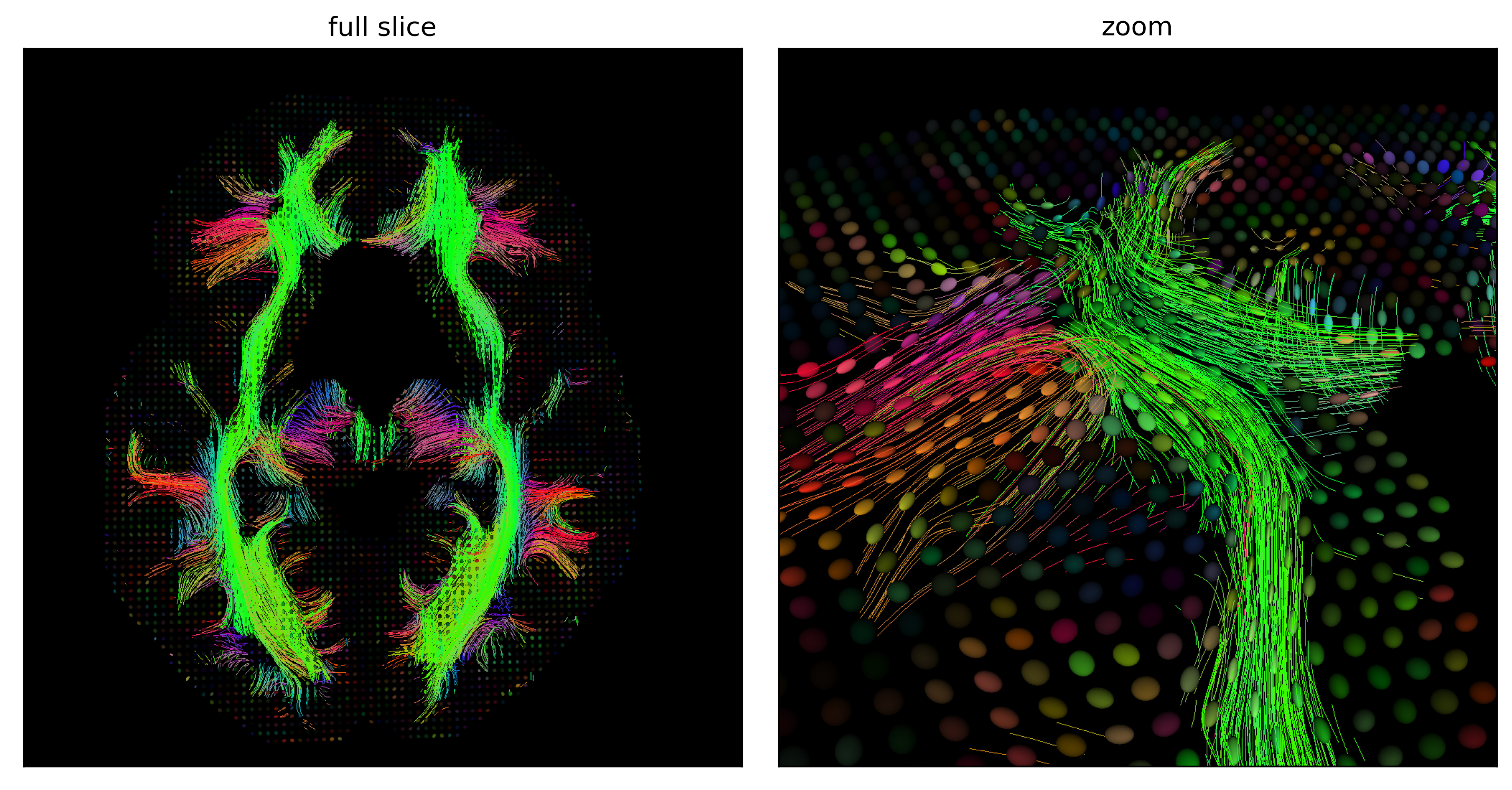
Fig. 53 Fibers reconstructed by a deterministic streamline approach, which consists in drawing a fiber following the principal direction of each tensor in an iterative way, starting from all the points in the white matter on an axial section (left) and zooming in on a portion of the cut (right). The color of each fiber codes for the main direction of diffusion along the fiber. Figure generated by python code adapted from a DIPY tutorial by P. Bellec under license CC-BY 4.0.¶

Tractography makes it possible to trace the path of white matter fibers in vivo. There are several approaches to tractography. Deterministic streamline tractography makes it possible to reconstruct white matter fibers starting from a given point in the white matter and moving iteratively along the main direction of diffusion. The path will end when we come to gray matter. This path will be traced using specific algorithms. Probabilistic tractography is similar to deterministic tractography, but also considers uncertainty about the direction of white matter fibers. So instead of reconstructing a single fiber associated with a point of white matter, probabilistic tractography will reconstruct several that will all be slightly different.

Preprocessing steps

Just like fMRI, registration and denoising steps are necessary to prepare the data before estimating the tensors and performing the tractography. Many parameters have to be selected for the tractography itself, which can influence the results. It is also necessary to select a white matter mask that contains the starting points for fiber reconstruction, obtained here by thresholding an AF map.

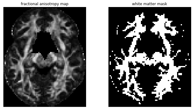
Fig. 54 Fractional anisotropic map (left) and white matter mask obtained by thresholding (right). Figure generated by python code adapted from a DIPY tutorial by P. Bellec under license CC-BY 4.0.¶

Fiber crossing¶

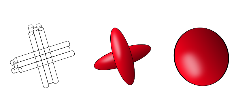
Fig. 55 Illustration of the fiber crossing problem, shown at left. The diffusion of water in each fiber is associated with a tensor that points in a different direction (middle). When we try to approximate the diffusion in the crossing with a single tensor, we observe an isotropic tensor (right). Figure by P Bellec, under license CC-BY 4.0, inspired by the thesis of C. Poupon, 1999.¶

A limitation we encounter with diffusion tensor imaging is fiber crossing. It is very common in white matter to have several intersecting fiber bundles. When many fibers cross as in the figure below, the diffusion tensor appears isotropic, even if there are indeed fibers present in the voxel. In this case, the fiber reconstruction algorithm will not know which direction to follow. One of the techniques used to solve this problem is high resolution diffusion imaging, which allows us to estimate several tensors for the same voxel. This technique consists of acquiring data in many directions (around 30 to 60 directions) using a HARDI sequence (High Angular Resolution Diffusion Imaging). The acquisitions made with this sequence are longer than those in DTI, 5-30 min vs 3-4 min.

from matplotlib import pyplot as plt
from dipy.reconst.csdeconv import auto_response_ssst
from dipy.reconst.csdeconv import ConstrainedSphericalDeconvModel
from dipy.data import default_sphere
from dipy.viz import actor

response, ratio = auto_response_ssst(gtab, maskdata, roi_radii=10, fa_thr=0.7)
csd_model = ConstrainedSphericalDeconvModel(gtab, response)
csd_fit = csd_model.fit(maskdata)
csd_odf = csd_fit.odf(default_sphere)
from dipy.data import default_sphere
fodf_spheres = actor.odf_slicer(csd_odf, sphere=default_sphere, scale=0.9,
                                norm=False, colormap='plasma')

# Create the 3D display.
scene = window.Scene()
scene.add(fodf_spheres)
scene.set_camera(position=(14.87946710578175, 25.770232149765413, 173.54578028650144),
                 focal_point=(33.43851200470716, 40.67356830562871, 15.545914873824975),
                 view_up=(0.003256400517440014, 0.9955397521536979, 0.09428678453221151))
window.record(scene, n_frames=1, out_path='../../../static/neuroscience/fodf-slice.png',
              size=(1000, 1000), reset_camera=False)
scene.set_camera(position=(6.398539759431944, 36.122368120824724, 21.074961978614017),
                 focal_point=(17.02336666201742, 55.39317316617157, 7.230217513090364),
                 view_up=(0.10205867972271891, 0.5426923506538308, 0.8337080055001721))
window.record(scene, n_frames=1, out_path='../../../static/neuroscience/fodf-zoom.png',
              size=(600, 600), reset_camera=False)   

# Make figure
from matplotlib import pyplot as plt
import imageio
fig1, ax = plt.subplots(1, 2, figsize=(12, 6), dpi=200,
                        subplot_kw={'xticks': [], 'yticks': []})
fig1.subplots_adjust(hspace=0.3, wspace=0.05)
im = imageio.imread('../../../static/neuroscience/fodf-slice.png')
ax.flat[0].imshow(im, interpolation='antialiased')
ax.flat[0].set_title('full slice')
im = imageio.imread('../../../static/neuroscience/fodf-zoom.png')
ax.flat[1].imshow(im, interpolation='none')
ax.flat[1].set_title('zoom')

# Glue the figure
from myst_nb import glue
glue("fodf-fig", fig1, display=False)

plt.close()

100%|███████████████████████████████████████████████████████████████████████████████████████| 24424/24424 [00:07<00:00, 3338.83it/s]

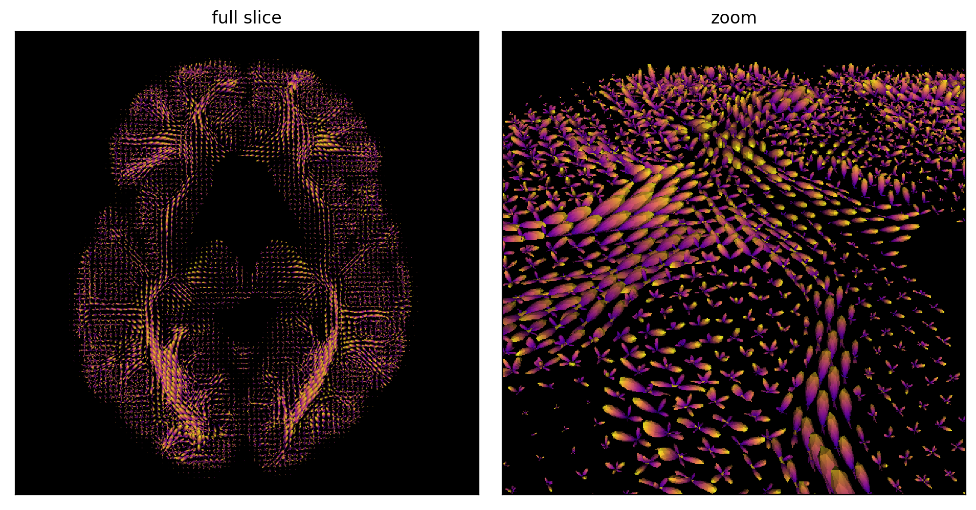
Fig. 56 Estimation of fODF on an axial slice (left) and zoom on a portion of the slice (right). Figure generated by python code adapted from a DIPY tutorial by P. Bellec under license CC- BY 4.0.¶

With a HARDI sequence, we can estimate a fiber Orientation Distribution Function (fODF) when there are perpendicular fiber crossings. This allows us to estimate several tensors inside a voxel and to overcome certain limits of the diffusion tensor (DTI). In areas with low anisotropy we observe several directions, like small balloons in each voxel, while we observe a main direction in the most important fibers.

csa_peaks = peaks_from_model(csd_model, maskdata[minx:maxx, miny:maxy, :, :], default_sphere,
                             relative_peak_threshold=.5,
                             min_separation_angle=15,
                             mask=mask_wm[minx:maxx, miny:maxy, :])

# Initialization of LocalTracking. The computation happens in the next step.
streamlines_generator = LocalTracking(csa_peaks, stopping_criterion, seeds,
                                      affine=affine, step_size=0.2, max_cross=5)
# Generate streamlines object
streamlines = Streamlines(streamlines_generator)

from dipy.viz import colormap
color = colormap.line_colors(streamlines)
streamlines_actor = actor.line(streamlines,
                               colormap.line_colors(streamlines))

# Create the 3D display.
scene = window.Scene()
scene.add(streamlines_actor)
scene.add(fodf_spheres)
scene.set_camera(position=(14.87946710578175, 25.770232149765413, 173.54578028650144),
                 focal_point=(33.43851200470716, 40.67356830562871, 15.545914873824975),
                 view_up=(0.003256400517440014, 0.9955397521536979, 0.09428678453221151))
window.record(scene, n_frames=1, out_path='../../../static/neuroscience/fibers-slice.png',
              size=(1000, 1000), reset_camera=False)
scene.set_camera(position=(6.398539759431944, 36.122368120824724, 21.074961978614017),
                 focal_point=(17.02336666201742, 55.39317316617157, 7.230217513090364),
                 view_up=(0.10205867972271891, 0.5426923506538308, 0.8337080055001721))
window.record(scene, n_frames=1, out_path='../../../static/neuroscience/fibers-zoom.png',
              size=(1000, 1000), reset_camera=False)

# Make figure
from matplotlib import pyplot as plt
import imageio
fig1, ax = plt.subplots(1, 2, figsize=(12, 6), dpi=300,
                        subplot_kw={'xticks': [], 'yticks': []})
fig1.subplots_adjust(hspace=0.3, wspace=0.05)
im = imageio.imread('../../../static/neuroscience/fibers-slice.png')
ax.flat[0].imshow(im, interpolation='antialiased')
ax.flat[0].set_title('full slice')
im = imageio.imread('../../../static/neuroscience/fibers-zoom.png')
ax.flat[1].imshow(im, interpolation='antialiased')
ax.flat[1].set_title('zoom')

# Glue the figure
from myst_nb import glue
glue("fodf-tracts-fig", fig1, display=False)

plt.close()

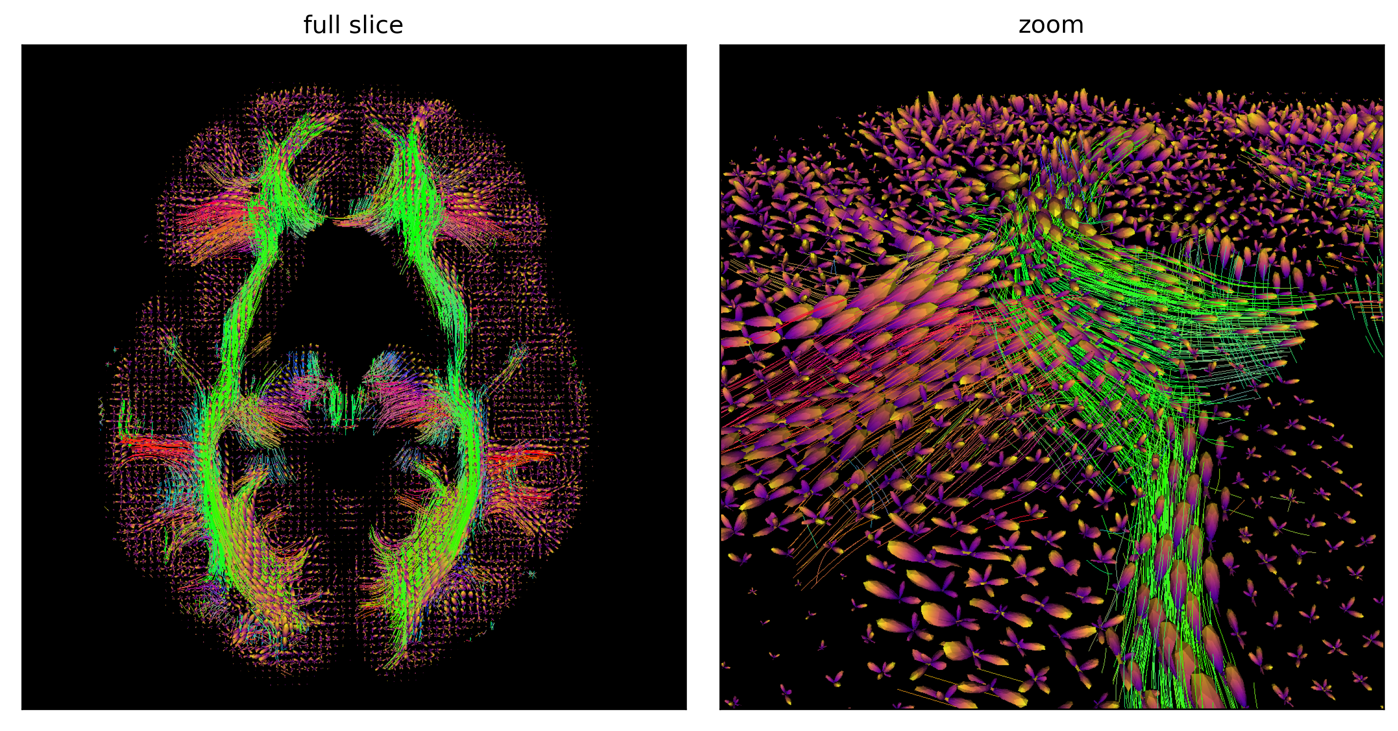
Fig. 57 Fibers reconstructed by a deterministic streamline approach with a multi-tensor approach, which makes it possible to follow several diffusion peaks at each voxel, from all the points in the white matter on an axial slice (left) and zoom on a portion of the cut (right). This approach makes it possible to be more robust to the presence of crossing fibers. Figure generated by python code adapted from a DIPY tutorial by P. Bellec under license CC-BY 4.0.¶

The ability of fODF to represent multiple tensors at each voxel allows the reconstruction of intersecting fibers, as is apparent in the zoom of Fig. 57. It is important to realize that the data used to generate Fig. 53 and Fig. 57 are the same, but the reconstructed fibers are very different! The parameters that we choose for the reconstruction method will also change the shape and the number of fibers. dMRI tractography is therefore not an exact science, and false positives (a reconstructed fiber that does not really exist) as well as false negatives (a fiber that is not reconstructed but which nevertheless exists) are very common.

Fiber Bundles¶

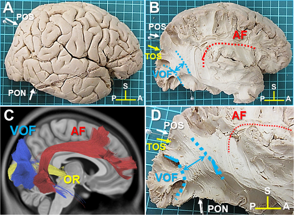
Fig. 58 Illustration of three fiber bundles: the radiating optics (OR), the arcuate fasciculus bundle (AF) and the vertical occipital bundle (VOF). The bundles are presented on different views of a dissection (A, B, D), as well as using a virtual dissection (C). Figure taken from [Jitsuishi et al., 2020], licensed under CC-BY 4.0.¶

We can provide tractography algorithms with priors about the fibers in the brain that we know from dissection studies. In a systematic reconstruction of fibers, everything will be traced, whereas in a virtual dissection, only certain bundles of fibers will be selected. These priors make it possible to limit false positives, and the use of high-performance tractography algorithms makes it possible to limit false negatives. There are a number of classic fiber bundles with well-established dissection patterns, such as the corpus callosum, the arcuate fasciculus bundle, or the superior longitudinal fascicle.

It is possible to calculate the average value of the fractional anisotropy, or any other metric, along a fiber, and then to compare this average value between different individuals to perform statistical tests. In this case, the registration between individuals is done via the identification of fiber bundles, rather than by a non-linear deformation method.

Conclusion¶

In this part of the course, we have seen the principles of diffusion MRI. Specifically, we have seen:

How to obtain dMRI images thanks to the diffusion of water in different directions.
How to estimate the diffusion process using tensors and measure different metrics (average diffusivity, fractional anisotropy).
The principle of tractography methods.
How to estimate fiber crossings.
How dMRI can be used to perform virtual dissection.

References¶

BFH+20: Mudathir Bakhit, Masazumi Fujii, Ryo Hiruta, Masayuki Yamada, Kenichiro Iwami, Taku Sato, and Kiyoshi Saito. The superior frontal longitudinal tract: a connection between the dorsal premotor and the dorsolateral prefrontal cortices. Scientific Reports, 10(1):15855, September 2020. Number: 1 Publisher: Nature Publishing Group. URL: https://www.nature.com/articles/s41598-020-73001-7 (visited on 2022-04-27), doi:10.1038/s41598-020-73001-7.
JHY+20: Tatsuya Jitsuishi, Seiichiro Hirono, Tatsuya Yamamoto, Keiko Kitajo, Yasuo Iwadate, and Atsushi Yamaguchi. White matter dissection and structural connectivity of the human vertical occipital fasciculus to link vision-associated brain cortex. Scientific Reports, 10(1):820, January 2020. Number: 1 Publisher: Nature Publishing Group. URL: https://www.nature.com/articles/s41598-020-57837-7 (visited on 2022-04-27), doi:10.1038/s41598-020-57837-7.

Exercices¶

In the following we created a few exercises that aim to recap core aspects of this part of the course and thus should allow you to assess if you understood the main points.

Exercise 6.1

Diffusion MRI can measure… (true/false, explain your answers)

An image with a tensor at each voxel.
An image with one or more tensors at each voxel.
A series of images sensitive to the diffusion of water in different directions.
Images showing the white matter fibers of the brain in 3D.

Exercise 6.2

Give an example of a region with…

Low fractional anisotropy, with high average diffusivity?
Strong fractional anisotropy, with low average diffusivity?
Low fractional anisotropy, with low average diffusivity?

Exercise 6.3

We observe a voxel whose fractional anisotropy is low. Give two interpretations of this observation.

Exercise 6.4

List three examples of fiber bundles.

Exercise 6.5

Give two examples of problems that can cause a deterministic streamline tractography process to fail.

Exercise 6.6

What is the advantage of performing group statistics on a fiber bundle, rather than voxel by voxel with traditional anatomical registration, as in fMRI?

Exercise 6.7

To answer the questions in this exercise, first read the article Quantification of apparent axon density and orientation dispersion in the white matter of youth born with congenital heart disease by Easson et al. (published in 2020 in the journal Neuroimage , volume 205, ID 116255). It is freely available at this address. The following questions require short-answer answers.

What type of participants were recruited in this study?
What is the main objective of the study?
What are the inclusion and exclusion criteria?
What neuroimaging technique is used? Is it a structural or functional technique?
What type of image acquisition sequence is used? List the parameters.
What types of analyzes have been applied?
Which figure (or table) meets the main objective of the study?
What is the main result of the study?

Spring/Fall term 2022

Diffusion MRI

Contents