Using Python for neuroimaging data - NiBabel
Contents
Using Python for neuroimaging data - NiBabel
The primary goal of this section is to become familiar with loading, modifying, saving, and visualizing neuroimages in Python. A secondary goal is to develop a conceptual understanding of the data structures involved, to facilitate diagnosing problems in data or analysis pipelines.
To these ends, we’ll be exploring the core python library for handling and wrangling neuroimaging data: nibabel. While this short introduction should get you started, it is well worth your time to look through nibabel's excellent documentation.
Nibabel
![]()
Nibabel is a low-level Python library that gives access to a variety of imaging formats, with a particular focus on providing a common interface to the various volumetric formats produced by MRI scanners and used in common neuroimaging toolkits such as FSL, AFNI, FreeSurfer and SPM:
NIfTI-1NIfTI-2SPM AnalyzeFreeSurfer.mgh/.mgzfilesPhilips
PAR/RECSiemens
ECATDICOM(limited support)
It also supports surface file formats:
GIFTIFreeSurfersurfaces,labelsandannotations
and others such as:
Connectivity
CIFTI-2
Tractography
TrackViz.trkfiles
as well as a number of related formats.
Note: Almost all of these can be loaded through the nibabel.load interface.
Setup
Before we actually start, we are going to need to import the nibabel library and a few others, more or less related to basic computing and plotting.
%matplotlib inline
from nilearn import plotting
import pylab as plt
import numpy as np
import nibabel as nb
Great, let’s get started.
Loading and inspecting images in nibabel
At first, we are going to explore how we can load and inspect neuroimages in nibabel. To this end, we will use parts of the tutorial datasets you should’ve downloaded during the course setup. Specifically, we are going to have a closer look at a functional MRI of sub-01. As mentioned before, basically all file formats are accessible via the nibabel load interface. All we need to do is to provide the path to the file we want to load:
img = nb.load('/data/ds000114/sub-01/ses-test/func/sub-01_ses-test_task-fingerfootlips_bold.nii.gz')
That’s all it takes and with that, we can directly inspect our now loaded fMRI image, for example via print which will give is the information stored in the header of the image:
print(img)
<class 'nibabel.nifti1.Nifti1Image'>
data shape (64, 64, 30, 184)
affine:
[[-3.99471426e+00 -2.04233140e-01  2.29353290e-02  1.30641693e+02]
 [-2.05448717e-01  3.98260689e+00 -3.10890853e-01 -9.74732285e+01]
 [ 6.95819734e-03  3.11659902e-01  3.98780894e+00 -8.06465759e+01]
 [ 0.00000000e+00  0.00000000e+00  0.00000000e+00  1.00000000e+00]]
metadata:
<class 'nibabel.nifti1.Nifti1Header'> object, endian='<'
sizeof_hdr      : 348
data_type       : b''
db_name         : b'?TR:2500.000 TE:50'
extents         : 0
session_error   : 0
regular         : b'r'
dim_info        : 0
dim             : [  4  64  64  30 184   1   1   1]
intent_p1       : 0.0
intent_p2       : 0.0
intent_p3       : 0.0
intent_code     : none
datatype        : int16
bitpix          : 16
slice_start     : 0
pixdim          : [-1.        4.        4.        3.999975  2.5       1.        1.
  1.      ]
vox_offset      : 0.0
scl_slope       : nan
scl_inter       : nan
slice_end       : 0
slice_code      : unknown
xyzt_units      : 10
cal_max         : 0.0
cal_min         : 0.0
slice_duration  : 0.0
toffset         : 0.0
glmax           : 255
glmin           : 0
descrip         : b''
aux_file        : b''
qform_code      : scanner
sform_code      : scanner
quatern_b       : 0.025633048
quatern_c       : -0.9989105
quatern_d       : -0.03895198
qoffset_x       : 130.6417
qoffset_y       : -97.47323
qoffset_z       : -80.646576
srow_x          : [-3.9947143e+00 -2.0423314e-01  2.2935329e-02  1.3064169e+02]
srow_y          : [ -0.20544872   3.982607    -0.31089085 -97.47323   ]
srow_z          : [ 6.9581973e-03  3.1165990e-01  3.9878089e+00 -8.0646576e+01]
intent_name     : b''
magic           : b'n+1'
This data-affine-header structure is common to volumetric formats in nibabel, though the details of the header will vary from format to format. As you can see above, the here utilized example entails information about the data shape, dimensions, affine, meta-data and much more. All of them are very useful and good to know (and should be identical to values indicated the corresponding json sidecar file if you use BIDS).
Question
Please have a look at each of the fields displayed above and try to answer the following questions:
what does the
valuerefer to?what does the respective
informationrepresent?
Accessing specific parameters
Seeing all these parameters entailed in the header we might want to evaluate and utilize some of them during various points of our analysis pipeline. With nibabel we can easily access all of them, either directly, e.g. the affine:
affine = img.affine
affine
array([[-3.99471426e+00, -2.04233140e-01,  2.29353290e-02,
         1.30641693e+02],
       [-2.05448717e-01,  3.98260689e+00, -3.10890853e-01,
        -9.74732285e+01],
       [ 6.95819734e-03,  3.11659902e-01,  3.98780894e+00,
        -8.06465759e+01],
       [ 0.00000000e+00,  0.00000000e+00,  0.00000000e+00,
         1.00000000e+00]])
or through the header object:
header = img.header['pixdim']
header
array([-1.      ,  4.      ,  4.      ,  3.999975,  2.5     ,  1.      ,
        1.      ,  1.      ], dtype=float32)
Note
Note that in the 'pixdim' above contains the voxel resolution (4., 4., 3.999), as well as the TR (2.5).
Furthermore, we can also access the underlying data of the image:
data = img.get_fdata()
data.shape
(64, 64, 30, 184)
Notes on working with neuroimaging and memory allocation
Why not just directly access the data via img.data? Working with neuroimages can use a lot of memory, so nibabel works hard to be memory efficient. If it can read some data while leaving the rest on disk, it will. img.get_data() reflects that it’s doing exactly that via some work behind the scenes.
Lets dive a bit further into this:
img.get_data_dtype()shows thetypeof thedataondiskimg.get_data().dtypeshows thetypeof thedatathat you’re working with
print((data.dtype, img.get_data_dtype()))
(dtype('<i2'), dtype('<i2'))
Even though true here, these are not always the same, and not being clear on this has caused problems. Further, modifying one does not update the other. This is especially important to keep in mind later when saving files.
What’s actually in the neuroimaging data?
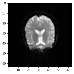
It might sound less crazy/fancy than you thought/hoped for but the data is a simple numpy array. It has a shape, it can be sliced and generally manipulated as you would any array as it contains numerical values in certain dimensions with certain expressions. Lets use matplotlib to visualize the data after directly accessing it via numpy to make this more clear:
plt.imshow(data[:, :, data.shape[2] // 2, 0].T, cmap='Greys_r')
print(data.shape)
(64, 64, 30, 184)
Question
Think about what the data and the respective values represents in terms of the discussed MRI principles and the signal we obtain through it.
Practical exercise 1:
How about some small practical exercise to further familiarize yourself with nibabel and neuroimaging data handling?
Please load the T1w data from subject 1 and then plot the image using the same volume indexing as before. Also, please print the shape of the data. Don’t worry if get stuck: just give it your best try and if it doesn’t work out, have a look at the solution below!
# work on solution here
Solution
t1 = nb.load('/data/ds000114/sub-01/ses-test/anat/sub-01_ses-test_T1w.nii.gz')
data = t1.get_data()
plt.imshow(data[:, :, data.shape[2] // 2].T, cmap='Greys_r')
print(data.shape)
Visually inspecting images via orthoview()
Nibabel has its own viewer, which can be accessed through img.orthoview() where img is the image you loaded via e.g. .load. It should present you with either 3 or 4 subplots for the respective dimensions, ie. 3 spatial (x, y, z) and in case of fMRI images 1 temporal(time indicated via TR). This viewer scales voxels to reflect their size, and label orientations.
Warning: img.orthoview() may not work properly on OS X.
Sidenote on plotting with orthoview()
As with other figures, f you initiated matplotlib with %matplotlib inline, the output figure will be static. If you use orthoview() in a normal IPython console, it will create an interactive window, and you can click to select different slices, similar to mricron or comparable viewers. To get a similar experience in a jupyter notebook, use %matplotlib notebook. But don’t forget to close figures afterward again or use %matplotlib inline again, otherwise, you cannot plot any other figures.
%matplotlib notebook
img.orthoview()
<OrthoSlicer3D: /data/ds000114/sub-01/ses-test/func/sub-01_ses-test_task-fingerfootlips_bold.nii.gz (64, 64, 30, 184)>
After we got a broad and general overview of neuroimaging data and what it entails, we should spend a bit more time on more precise aspects of neuroimaging data and its handling using nibabel. Specifically, we will spend a closer look at the header and the affine. Please note that we will be using the t1w data of sub-01 for this part. Thus, if you didn’t went through the previous exercise, you should do so now or make sure to check/run the solution. To make sure everything works, please try to use .orthoview() to plot and investigate the t1w image.
Solution
t1.orthoview()
Header
The header is a general property of neuroimaging data in most file formats and in nibabel the structure that stores all of the metadata of the image. As indicated above, you can query it directly, if necessary. For example, getting the description:
t1.header['descrip']
array(b'FSL5.0', dtype='|S80')
But it also provides interfaces for the more common information, such as get_zooms, get_xyzt_units, get_qform, get_sform which respectively provide spatial, temporal and affine information of the image at hand:
t1.header.get_zooms()
(1.0, 1.2993759, 1.0)
t1.header.get_xyzt_units()
('mm', 'sec')
t1.header.get_qform()
array([[ 9.99131938e-01, -5.16292391e-02,  1.25136054e-02,
        -1.25263863e+02],
       [ 4.07721521e-02,  1.29202043e+00, -9.81179047e-02,
        -7.31330109e+01],
       [-8.54416425e-03,  1.28044319e-01,  9.95096119e-01,
        -1.77554291e+02],
       [ 0.00000000e+00,  0.00000000e+00,  0.00000000e+00,
         1.00000000e+00]])
t1.header.get_sform()
array([[ 9.99131918e-01, -5.16291820e-02,  1.25127016e-02,
        -1.25263863e+02],
       [ 4.07721959e-02,  1.29202044e+00, -9.81179178e-02,
        -7.31330109e+01],
       [-8.54506902e-03,  1.28044292e-01,  9.95096147e-01,
        -1.77554291e+02],
       [ 0.00000000e+00,  0.00000000e+00,  0.00000000e+00,
         1.00000000e+00]])
Speaking of the affine, lets check it out in more detail:
Affine
In our case, the affine refers to a 4 x 4 numpy array. This describes the transformation from the voxel space (indices [i, j, k]) to the reference space (distance in mm (x, y, z)).
It can be used, for instance, to discover the voxel that contains the origin of the image:
x, y, z, _ = np.linalg.pinv(affine).dot(np.array([0, 0, 0, 1])).astype(int)

print("Affine:")
print(affine)
print
print("Center: ({:d}, {:d}, {:d})".format(x, y, z))
Affine:
[[-3.99471426e+00 -2.04233140e-01  2.29353290e-02  1.30641693e+02]
 [-2.05448717e-01  3.98260689e+00 -3.10890853e-01 -9.74732285e+01]
 [ 6.95819734e-03  3.11659902e-01  3.98780894e+00 -8.06465759e+01]
 [ 0.00000000e+00  0.00000000e+00  0.00000000e+00  1.00000000e+00]]
Center: (31, 27, 18)
The affine also encodes the axis orientation and voxel sizes:
nb.aff2axcodes(affine)
('L', 'A', 'S')
nb.affines.voxel_sizes(affine)
array([3.99999995, 4.00000009, 3.99997491])
nb.aff2axcodes(affine)
('L', 'A', 'S')
nb.affines.voxel_sizes(affine)
array([3.99999995, 4.00000009, 3.99997491])
Normally, we’re not particularly interested in the header or the affine. But it’s important to know they’re there. And especially, to remember to copy them when making new images or working with derivatives, so that they stay aligned with the original image (if required).
Now you might think: it seems a bit cumbersome to get/access all that information to e.g. check and/or evaluate a given image. First of all: come on, it’s just a few lines of rather simple code. Second, if you really don’t want to fire up a python session and run a few commands/functions: nibabel also has your back here.
nib-ls
Nibabel comes packaged with a command-line tool called nib-lis to print common metadata about any (volumetric) neuroimaging format nibabel supports. By default, it shows (on-disk) data type, dimensions and voxel sizes. Lets try it out via using the fMRI data of sub-01 again:
!nib-ls /data/ds000114/sub-01/ses-test/func/sub-01_ses-test_task-fingerfootlips_bold.nii.gz
/data/ds000114/sub-01/ses-test/func/sub-01_ses-test_task-fingerfootlips_bold.nii.gz int16 [ 64, 64, 30, 184] 4.00x4.00x4.00x2.50 sform
We can also inspect header fields by name, for instance, descrip:
!nib-ls -H descrip /data/ds000114/sub-01/ses-test/anat/sub-01_ses-test_T1w.nii.gz
/data/ds000114/sub-01/ses-test/anat/sub-01_ses-test_T1w.nii.gz float32 [256, 156, 256] 1.00x1.30x1.00 b'FSL5.0' sform
This concludes the basic neuroimaging data exploration section which discussed commands and functions should already allow you to do a lot of common tasks and work with neuroimaging data. However, there’s obviously way more to it. For example, creating and saving images.
Creating and saving images
Suppose we want to save space by rescaling our image to a smaller datatype, such as an unsigned byte. To do this, we first need to take the data, change its datatype and save this new data in a new NIfTI image with the same header and affine as the original image. At first, we need to load the image and get the data (using the fMRI data of sub-01 once more):
img = nb.load('/data/ds000114/sub-01/ses-test/func/sub-01_ses-test_task-fingerfootlips_bold.nii.gz')
data = img.get_fdata()
Now we force the values to be between 0 and 255 and change the datatype to unsigned 8-bit:
rescaled = ((data - data.min()) * 255. / (data.max() - data.min())).astype(np.uint8)
Now we can save the changed data into a new NIfTI file:
new_img = nb.Nifti1Image(rescaled, affine=img.affine, header=img.header)
nb.save(new_img, 'rescaled_image.nii.gz')
Let’s look at the datatypes of the data array, as well as of the nifti image:
print((new_img.get_fdata().dtype, new_img.get_data_dtype()))
(dtype('float64'), dtype('<i2'))
That’s not optimal. Our data array has the correct type, but the on-disk format is determined by the header, so saving it with img.header will not do what we want. Also, let’s take a look at the size of the original and new file.
orig_filename = img.get_filename()
!du -hL rescaled_image.nii.gz $orig_filename
 12M	rescaled_image.nii.gz
 24M	/data/ds000114/sub-01/ses-test/func/sub-01_ses-test_task-fingerfootlips_bold.nii.gz
So, let’s correct the header issue with the set_data_dtype() function:
img.set_data_dtype(np.uint8)
and then saving image again:
new_img = nb.Nifti1Image(rescaled, affine=img.affine, header=img.header)
nb.save(new_img, 'rescaled_image.nii.gz')
After which we evaluate our image again:
print((new_img.get_fdata().dtype, new_img.get_data_dtype()))
(dtype('float64'), dtype('uint8'))
Perfect! Now the data types are correct. And if we look at the size of the image we even see that it got a bit smaller.
!du -hL rescaled_image.nii.gz
10M rescaled_image.nii.gz
Conclusions
In this first introduction of how to work with neuroimaging data using python, we’ve explored loading, saving and visualizing neuroimages via nibabel, as well as how it can make some more sophisticated manipulations easy. At this point, you should be able to inspect and plot most images you encounter, as well as make modifications while preserving the alignment (at least for basic operations).