Magnetic Resonance Imaging (MRI)
Contents
Magnetic Resonance Imaging (MRI)
Objectives 📍
This part of the course aims to introduce you to the physical principles of magnetic resonance imaging. During this part of the course, we will cover four fundamental principles of MRI:
Magnetic resonanceRelaxation: parametersT1andT2ImagingMRI sequences
Anatomy of an MRI
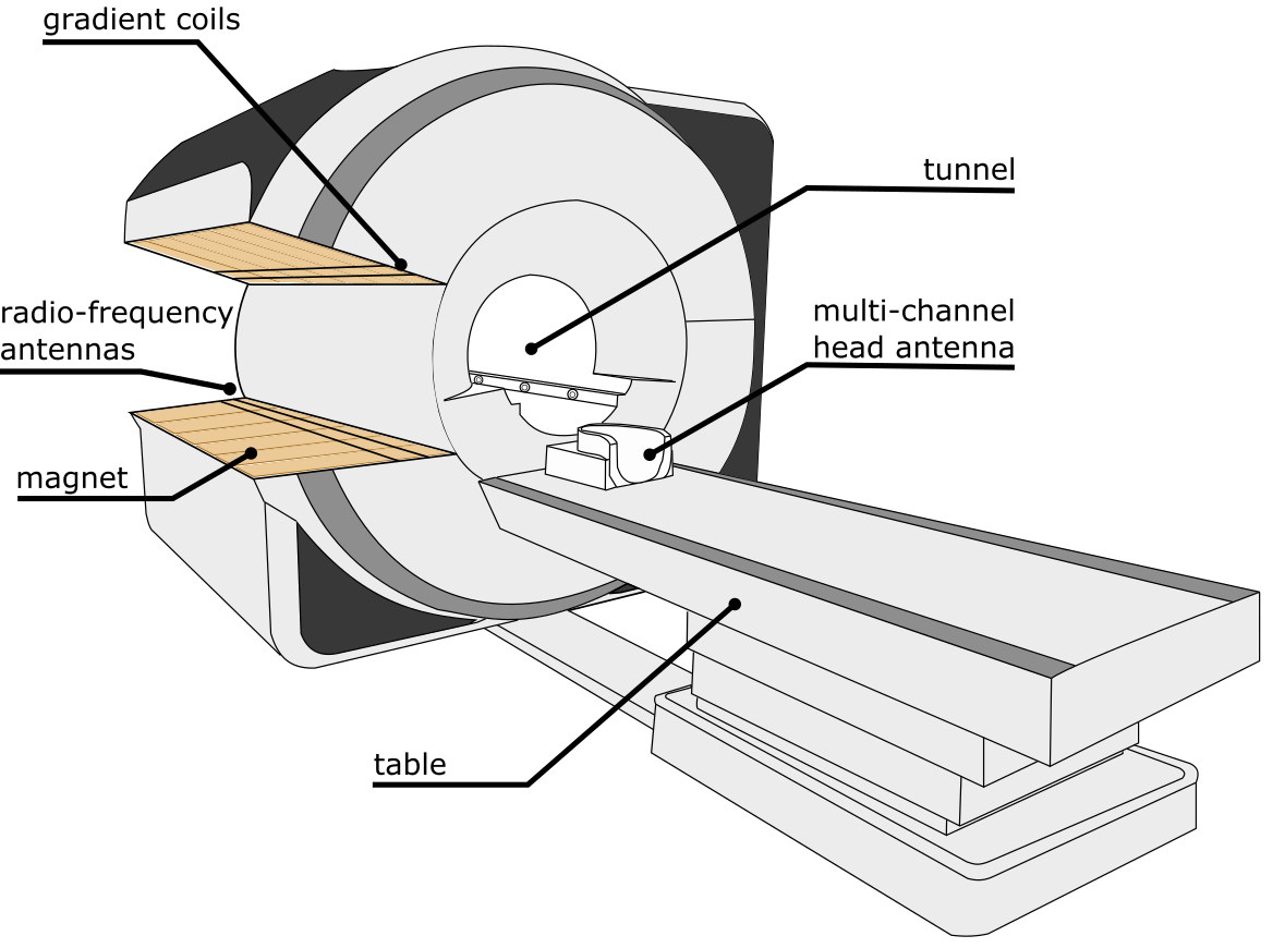
Fig. 16 Schematic illustration of the main components of an MRI machine. Figure generated by P. Bellec, 2021, licensed under CC-BY.
Fig. 16 allows us to observe the main elements of an MRI device, and in particular:
The magnet: this is a
coilthat generates a very strongmagnetic field. Thiscoilis immersed inliquid helium, close to absolute zero, which makes itsuperconductive: theelectric currentwhich crosses it does not undergo any loss of energy, and can continue to circulate for a very long time. For this reason, theMRI magnetcontinues to operate continuously, even when the machine is not in use.The gradient coils: allow to vary the
intensityof themagnetic fieldin space. Duringimage acquisition, thegradientsare activated and then stopped several times.Gradientscan be produced in any direction.The radio-frequency antenna: makes it possible to (1)
excitematterusingtransmitters, and (2) measure theresponseof thesebiological tissuestoexcitationusingreceivers. Theradio-frequency pulsesgenerated by theantennacreate a weakmagnetic fieldperpendicularto the mainmagnetic fieldgenerated by themagnet. Receivingantennascan also be placed in specific headgear.
We’ll talk more about how all of these work in the next few sections.
Warning
MRI is very sensitive to head movements! Cushions or other devices can be used to reduce movement.
Note
Coil + current = magnetic field!
By creating a ring with electric wire and passing an electric current, we produce a magnetic field. In the video below we can see the magnetic field lines being drawn when the magnetic field is activated. Field lines are straight as they pass through the center of the ring, but they propagate in circles away from the center of the ring. To obtain a constant magnetic field inside the ring, we can thicken the ring so as to form a cylinder. It’s the same principle that we find in an MRI machine!
from IPython.display import HTML
import warnings
warnings.filterwarnings("ignore")

# Youtube
HTML('<iframe width="560" height="315" src="https://www.youtube.com/embed/bq6IhapfucE" title="YouTube video player" frameborder="0" allow="accelerometer; autoplay; clipboard-write; encrypted-media; gyroscope; picture-in-picture" allowfullscreen></iframe>')
Magnetic spin and B0 field
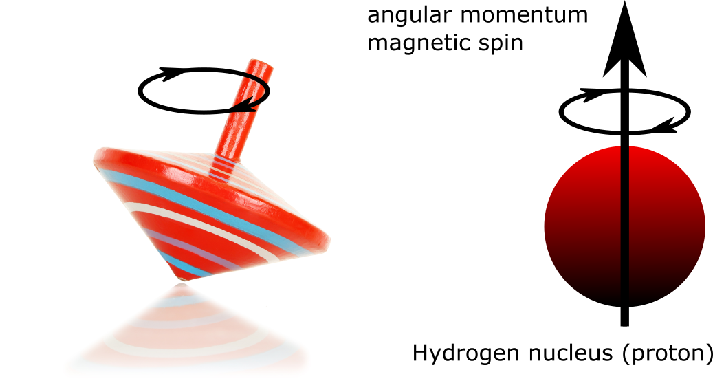
Fig. 17 A proton is like a small magnet, whose magnetic field oscillates around a given position (precessional motion), and is characterized by angular momentum, or spin. The right part of the figure was generated by P. Bellec, 2021, under CC-BY license. The left part of the figure is adapted from an image shutterstock ID 130826045, used under standard shutterstock license.
The protons that make up part of the atoms behave like little magnets that spin around their own axis, similar to a spinning top (see Fig. 17). This rotation of the magnetic moment is called the precession movement and depends among other things on the composition of the core. Thus, each type of nucleus has a characteristic Larmor frequency.
Note
A hydrogen atom has a Larmor frequency of 42.58 MHz/Tesla. This frequency is therefore not fixed, but depends on the strength of the magnetic field! Placed in an external magnetic field of 1T, a hydrogen atom rotates 42580000 times per second. The stronger the magnetic field in which a proton is located, the more the speed at which the magnetic moment of this proton rotates will increase.
The MRI magnet helps align the magnetic moment of the protons along the same axis as the main magnetic field, called B0. This B0 field goes from the feet to the head. The strength of the main magnet is measured in Teslas (T). 1.5T devices are mainly used for clinical purposes, while in research, the standard is rather 3T, which is about 60,000 times more powerful than the Earth’s magnetic field! The 7T devices represent today the new frontier used in research, and some 10T+ devices exist in the world. But why would we want to increase the strength of the magnetic field? By increasing the strength of the magnetic field, we can gain spatial and temporal resolution. On the other hand, increasing the strength of the magnetic field can also introduce artifacts!
Magnetic resonance
Note
Resonance… not just magnetic
We find resonance phenomena in many situations. A known example is the resonance between the wind and the Tacoma Bridge, which led to the collapse of the bridge (see the video below).
from IPython.display import HTML
import warnings
warnings.filterwarnings("ignore")

# Youtube
HTML('<iframe width="560" height="315" src="https://www.youtube.com/embed/3mclp9QmCGs" title="YouTube video player" frameborder="0" allow="accelerometer; autoplay; clipboard-write; encrypted-media; gyroscope; picture-in-picture" allowfullscreen></iframe>')
We can think of resonance as a seesaw motion. If we push the swing randomly, it won’t swing much. To have an amplified swing motion, we need to push the swing at the same frequency as the natural frequency of the swing. We will then enter into resonance with the swing, and its movement will amplify. We can therefore see the swing as a phenomenon of resonance between the object that is swinging and the person who gives impetus to this object.
MRI exploits this resonance phenomenon. The radio-frequency (RF) antenna creates a series of radio-frequency waves in the direction perpendicular to the B0 field, ie in the direction of the B1 field. By producing a series of pulses following the Larmor frequency of hydrogen, the hydrogen atoms come into resonance and tilt in the perpendicular direction.
By stopping the pulses, the hydrogen atoms enter into relaxation, that is to say that their magnetic moment will return to the initial direction B0. In other words, the magnetic moment in direction B1 decreases to return in direction B0. This relaxation phenomenon is very important, because the speed of relaxation will depend on the characteristics of the tissues that have been excited. The relaxation speed is measured by the receiving antennas placed in the helmet around the participant’s head!
Note
It is important to understand that the signal we measure in MRI does not come from a single proton. For reference, 18 grams of water contains one mole of H2O molecules, or about \(10^{24}\) hydrogen atoms… The signal that we are measuring comes from the juxtaposition of the spins of all of these atoms. A radio-frequency wave which resonates with hydrogen will not only tilt the spins, but also bring them into phase. Imagine that you have a thousand swings, which you push at the same time (at the right frequency). Not only will the movement of the swings gain in amplitude, but all the swings will be at the same point in their trajectory at the same time. It is the same for spins after an excitement.
Note
Why radio?
As we have seen, the Larmor frequency of hydrogen is 42.58 MHz/Tesla. In a 3T MRI, we are therefore going to excite with a wave at a frequency of approximately 120 MHz, or 120 million waves per second (!). This type of frequency falls into the domain of radio waves.
Section selection and image formation
We have seen how a radio-frequency wave can excite hydrogen nuclei and measure the response to this excitation to examine the characteristics of tissues. But how to make an image? The gradient coils make it possible to vary the amplitude of the magnetic field in three directions:
Direction z: fromfeettoheadDirection x: fromlefttorightDirection y: from thebackof theheadto thenose
These variations are much weaker than the B0 field, and only represent a fraction of a Tesla, but this will allow us to extract spatial information in a resonance process. Using these gradients, it is possible to measure the magnetic properties of tissues located at a specific point in space, and therefore to make a (3D) image. This process is complex, but the first step is relatively simple to understand: it is the cut selection.
We remember that the Larmor frequency of a particle depends on the strength of the magnetic field in which it finds itself. By changing the strength of the magnetic field in a given direction thanks to the gradient coils, we are going to modify the Larmor frequency of the hydrogen atoms at a specific point in the gradient. The radio-frequency pulses will only excite the hydrogen atoms in the cut where the magnetic field has the strength that corresponds to the excitation frequency. In this way, instead of receiving signal from the whole brain, we only receive signal from the selected slice, because only the hydrogen atoms in this slice will resonate.
We still have to cut our section into pixels… But that is largely beyond the context of this introductory chapter. To learn more about spatial encoding in MRI, you can consult this resource.
Note
Field of View (FOV)
When we make a 3D image of the brain, we will slice the brain into a series of slices. By knowing the size of the cuts as well as the number of cuts, we can deduce the size of the 3D cube that corresponds to the image. This size is called field of view, or FOV.
Note
The MRI: a noisy machine
The acquisition of an image requires modifying the gradients quickly. The rapid current changes in the gradient coils, as well as in the radio-frequency wave emitting coils, cause the coils to expand and contract rapidly. These movements create significant noise. Each type of image has its own “music”, which depends on the nature and order of the excitations and gradients. See excerpts below.
from IPython.display import HTML
import warnings
warnings.filterwarnings("ignore")

# Youtube
HTML('<iframe width="560" height="315" src="https://www.youtube.com/embed/9GZvd_4ot04?start=11" title="YouTube video player" frameborder="0" allow="accelerometer; autoplay; clipboard-write; encrypted-media; gyroscope; picture-in-picture" allowfullscreen></iframe>')
\(T_1\) and \(T_2\) contrasts
The contrasts \(T_1\) and \(T_2\) are the main parameters acquired during an MRI session. Initially, the hydrogen proton spins are aligned with the \(B_0\) field. The application of radio-frequency pulses causes the spins to tilt along the \(B_1\) axis, an axis perpendicular to \(B_0\). Once the radio-frequency pulses have stopped, the spins realign with the \(B_0\) field. This realignment is characterized by two distinct dynamics, linked to the time constants \(T_1\) and \(T_2\).
Contrast in \(T_1\). The increase in the component according to \(B_0\) (component \(M_z\)), or longitudinal relaxation, follows an increasing exponential function. The characteristic time of this growth (the speed of growth) is called \(T_1\). The time \(T_1\) corresponds to the time elapsed to obtain 63% of the equilibrium value of the magnetic moment contribution along the z axis (\(M_0\)). For those who are comfortable with mathematical expressions, the regrowth in \(B_0\) follows the equation \(M_z(t) = M_0 ( 1 - e^{-t / T_1})\).
# ignore warnings
import warnings
warnings.filterwarnings("ignore")

# import necessary libraries
import matplotlib.pyplot as plt
import numpy as np
from myst_nb import glue

# setup figures
fig = plt.figure(figsize=(15, 5))

# Exponential functions for T1 curves (for example only)
t = np.linspace(0,5,100)
y1 = 70 * (1 - np.exp(-t / 1.2))
y2 = 85 * (1 - np.exp(-t / 1.3))
y3 = 100 * (1 - np.exp(-t / 1.5))

# Trace the figure
ax_plot = plt.subplot(1, 3, 1)
plt.plot(t, y1, label="Cerebrospinal fluid")
plt.plot(t, y2, label="grey matter")
plt.plot(t, y3, label="white matter")
plt.vlines(1, 0, 60, colors="black", linestyles="--")
plt.text(1, 60, "TE")
plt.vlines(4, 0, 60, colors="black", linestyles="--")
plt.text(4, 60, "TR")
plt.xlabel("Time", loc="right")
plt.ylabel("mz", loc="top")
plt.title("Curve in T1")
plt.legend()
plt.gca().axes.yaxis.set_ticklabels([])
plt.gca().axes.xaxis.set_ticklabels([])

# Import required modules and dataset
from nilearn.datasets import fetch_icbm152_2009
from nilearn.plotting import plot_anat

data_mri = fetch_icbm152_2009()

# display T1-weighted image
ax_plot = plt.subplot2grid((1, 3), (0, 1), colspan=2)
plot_anat(data_mri.t1, figure=fig, title="MRI - T1 contrast", axes=ax_plot,
    cut_coords=[-17, 0, 17])

glue("relax-t1-fig", fig, display=False)
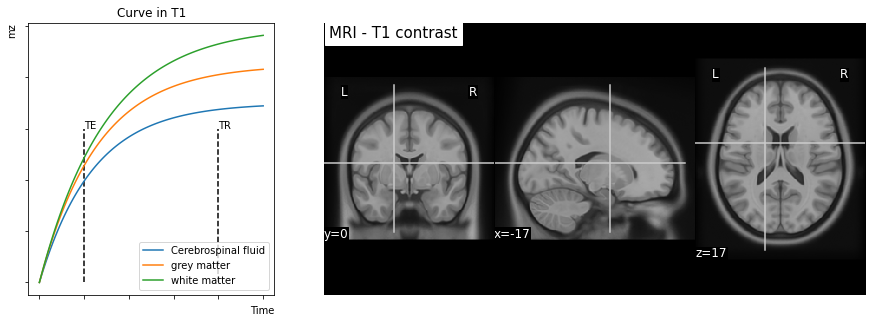
Fig. 18 Longitudinal relaxation and contrast \(T_1\). Left image: growth of the magnetic field along the \(B_0\) axis, called \(M_{z}\). Note that different tissue types exhibit distinct longitudinal relaxation curves. Right image: an image generated by reading at time \(TE\) presents a contrast between the different tissue types. This figure is generated by python code, click on the + to see the code.
Note
At equilibrium, the contribution of the magnetic moment along the \(B_0\) axis is called \(M_0\). This value depends on the density of protons in the tissues, i.e. the number of hydrogen atoms present in the tissue. Thus, from one voxel to another, we do not necessarily obtain the same value of \(M_0\). It is possible to image this parameter, and we then speak of an image in proton density.
Contrast in \(T_2\). The decrease in the component according to \(B_1\) (component \(M_{xy}\)), or transverse relaxation, follows a decreasing exponential function. The characteristic time of this decrease (the speed of decrease) is called \(T_2\). The time \(T_2\) corresponds to the time elapsed to obtain 37% of the value of the contribution of the initial magnetic moment along the axis \(B_1\). For those who are comfortable with mathematical expressions, the decrease in \(B_1\) follows the equation \(M_{xy}(t) = M_1 e^{-t / T_2}\). The constant \(M_1\) will depend, among other things, on the density of protons, like \(M_0\), and will vary from one tissue to another.
# ignore warnings
import warnings
warnings.filterwarnings("ignore")

# import necessary functions
import matplotlib.pyplot as plt
import numpy as np
from myst_nb import glue

# setup the figure
fig = plt.figure(figsize=(15, 5))

# Exponential functions for T2 curves (for example only)
t = np.linspace(0, 5, 100)
y1 = 100 * np.exp(-t / 1.5)
y2 = 85 * np.exp(-t / 1.1)
y3 = 70 * np.exp(-t / 0.8)

# Tracer la figure
ax_plot = plt.subplot(1, 3, 1)
plt.plot(t, y1, label="Cerebrospinal fluid")
plt.plot(t, y2, label="grey matter")
plt.plot(t, y3, label="white matter")
plt.vlines(1, 0, 60, colors="black", linestyles="--")
plt.text(1.1, 60, "TE")
plt.vlines(4, 0, 60, colors="black", linestyles="--")
plt.text(4, 60, "TR")
plt.xlabel("Time", loc="right")
plt.ylabel("Mz", loc="top")
plt.title("Curve in T2")
plt.legend()
plt.gca().axes.yaxis.set_ticklabels([])
plt.gca().axes.xaxis.set_ticklabels([])

# Import required modules and dataset
from nilearn.datasets import fetch_icbm152_2009
from nilearn.plotting import plot_anat

data_mri = fetch_icbm152_2009()

# display the T2-weighted image
ax_plot = plt.subplot2grid((1, 3), (0, 1), colspan=2)
plot_anat(data_mri.t2, figure=fig, title="MRI - T2 contrast", axes=ax_plot,
    cut_coords=[-17, 0, 17])

glue("relax-t2-fig", fig, display=False)
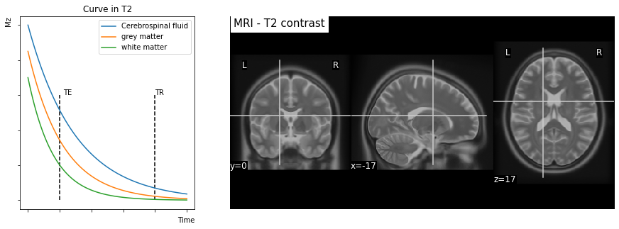
Fig. 19 Transverse relaxation and contrast \(T_2\). Left image: decrease of the magnetic field along the \(B_1\) axis, called \(M_{xy}\). Note that different tissue types exhibit distinct transverse relaxation curves. Right image: an image generated by reading at time \(TE\) presents a contrast between the different tissue types. This contrast is essentially reversed with respect to contrast \(T_1\). This figure is generated by python code, click on the + to see the code.
Note
\(TE\)
When we acquire MRI data, we generally do not measure the entire relaxation curve, but simply a measurement point at time \(TE\). By choosing the \(TE\) appropriately, we will obtain very different reading values for the different tissues. The time \(TE\) will be different for a contrast \(T_1\) and a contrast \(T_2\).
Note
\(TR\)
We call \(TR\) the time which separates two series of excitations. This value will correspond to the acquisition time of a section for a structural MRI, and the acquisition time of a complete cerebral volume in fMRI. It’s a weird convention, but widely used by MRI physicists.
Note
flip angle
If we’re interested in the end of the relaxation process, we don’t need to flip the spins completely in the \(B_1\) direction, just a certain number of degrees from \(B_0\). This parameter is called flip angle.
\(T_2^*\), fMRI, dMRI
Phase shift. As we saw in the sidebar on phase, the radio-frequency pulses will not only flip the spins, but also bring them into phase. When we stop the impulses, the spins will gradually go out of phase. This phase shift is due to micro-interactions between protons as well as tissue molecules that exhibit magnetic properties. The relaxation curve will have the same shape, but with modified characteristic times, which we call \(T_1^*\) and \(T_2^*\).
Functional MRI. The inhomogeneities in the magnetic field which cause the phase shift can in particular be created by the deoxyhemoglobin that we find in the blood. We will see in more detail how oxyhemoglobin and deoxyhemoglobin disturb the magnetic field in the chapter on functional MRI. In functional MRI, we use T2*-weighted sequences.
Diffusion MRI. In diffusion MRI, we also use the T2* contrast. On the other hand, in diffusion MRI, we measure inhomogeneities by alternating the direction of the pulses (eg by giving a pulse along the xy axis, then by giving a pulse along the -xy axis). By taking several images with different directions of excitation, we can get an idea of the direction of water diffusion. This operation allows us in the end to know the direction of the fibers of white matter, because the more a fiber points towards a given direction, the greater the diffusion will be in this direction. We will come back to this subject in the chapter on diffusion MRI.
Console and acquisition sequences
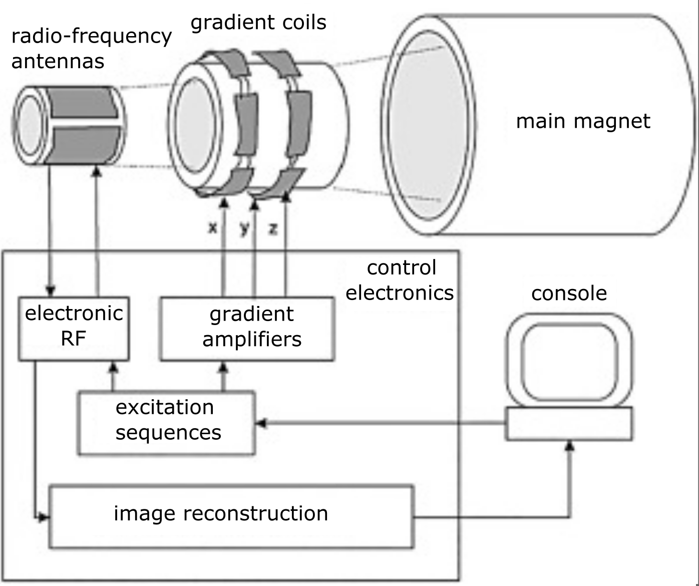
Fig. 20 Connections between the console and the different parts of an MRI system. Figure adapted by P. Bellec, 2021, licensed under CC-BY. The original Figure is taken from the article by [Gruber et al., 2018], licensed under CC-BY-NC.
All elements of the MRI device can be controlled by the console (see Fig. 20). We have seen together the key principles of MRI, but an actual image is acquired with a complex series of excitations and measurements, which is called an acquisition sequence. Once the sequence has been programmed, we can always modify certain parameters of the sequence, such as:
\(TE\)
\(TR\)
field of view(FOV)NumberofcutsThicknessofcutsVoxel size
Conclusions
This chapter introduced you to the physical principles of MRI. We have seen the different components of an MRI machine, the different magnetic phenomena allowing us to acquire images, as well as some parameters that we can modify during the acquisition of MRI data. In the next chapter, we will talk about morphometry using structural MRI.
References
- 1
Bernhard Gruber, Martijn Froeling, Tim Leiner, and Dennis W.J. Klomp. RF coils: A practical guide for nonphysicists. Journal of Magnetic Resonance Imaging, 48(3):590–604, 2018. _eprint: https://onlinelibrary.wiley.com/doi/pdf/10.1002/jmri.26187. URL: https://onlinelibrary.wiley.com/doi/abs/10.1002/jmri.26187 (visited on 2022-04-01), doi:10.1002/jmri.26187.
Exercices
In the following we created a few exercices that aim to recap core aspects of this part of the course and thus should allow you to assess if you understood the main points.
Exercice 2.1
Rank the characteristic times in ascending order, if possible.
TEvsTRTRvs.T1T1vs.TE
Exercice 2.2
True or false? The field strength of an MRI is related to the size of the MRI.
Exercice 2.3
Choose between the correct answer from 1, 2 or 3. the spin of a hydrogen proton has…
A fixed
rotational frequencyis theLarmor frequencyA
variable rotation frequencyA
rotational frequencythat depends on thestrengthof themagnetic fieldin theMRI.
Exercice 2.4
What produces noise in an MRI acquisition?
The
B0fieldAir conditioningtocoolthemagnetGradient coilsThe
radio-frequency antenna
Exercice 2.5
True or false? The MRI magnet consumes a lot of electricity.
Exercice 2.6
True or false? Functional MRI and diffusion MRI both use T2* contrast.
Exercice 2.7
In an anatomical image, we see white ventricles on a black background. Is this a T1- or T2-weighted acquisition? Explain why.
Exercice 2.8
We decide to modify an MRI sequence to reduce the flip angle: the spins will tilt by 70 degrees, instead of 90 degrees. What will be the effect on the TR of this change?
Exercice 2.9
A T1 acquisition is performed with a field of view of 210 mm x 210 mm in-plane, and a resolution of 1 mm x 1 mm in the slice. What is the cut size (number of pixels x number of pixels)?
Exercice 2.10
An fMRI acquisition is carried out with a resolution of 3 mm ×3 mm in the slice, a slice of dimension 64×64, a slice thickness of 3.4 mm with 31 slices. We have a TR of 2 seconds, and we acquire 150 volumes.
What is the size of the 3D field of view, knowing that the slices are acquired in the axial plane?
What is the duration of the acquisition?
Exercice 2.11
To answer this question, read the article by Shukla et al, “Aberrant Frontostriatal Connectivity in Negative Symptoms of Schizophrenia”, published in Schizophrenia Bulletin (2019, 45(5): 1051-59) and available open access at this address. The following questions require short answers.
What is the
strengthof theMRI magnet?How many
channelsare present in thehead antenna?What is the
TRofstructural acquisition? andfunctional acquisition? Comparing these two times with each other, does it make sense that one is bigger than the other?What is the name of the
sequenceused forstructural acquisition?What is the name of the
sequenceused forfunctional acquisition?What is the
TEof thestructural acquisition? andfunctional acquisition? Comparing these two times with each other, does it make sense that one is bigger than the other?What is the
sizeof thefunctional acquisitionfield of view, incm?How many
brain volumesareacquiredduring thefunctional sequence?
Exercice 2.12
We want to isolate the thalamus on an individual anatomical image. Which contrast should we use: T1, T2 or both? Please justify your answer.