Morphometric analyzes¶

Objectives 📍¶

This part of the course introduces different approaches to quantifying brain morphology using anatomical magnetic resonance imaging data. This chapter discusses three major analytical approaches:

volumetry, which aims to measure the size of a brain region;
voxel-based morphometry or VBM*, which aims to measure the volume of local gray matter for each voxel in the brain;
Surface analyses, which exploit the ribbon structure of gray matter to measure thickness and cortical surface area.

We will also talk about image analysis steps useful for all of these techniques: registration, segmentation, smoothing and quality control .

Morphometry¶

Fig. 21 Study of Dürer on the proportions of the face. Public domain image taken from wikimedia.¶

In neuroscience, morphometry is the study of the shape of the brain and its structures. The term morphometry combines two terms taken from ancient Greek: *morphos* (form) and *metron* (measurement). Morphometryis therefore the "measurement" of the "shape". To measure theshapeof thebrain, it is necessary to be able to clearly observe the neuroanatomical boundaries. Anatomical MRIgives us a good contrast betweengray matter, white matterandcerebrospinal fluid. Combined with automatic image analysis tools, MRItherefore makes it possible to carry outcomputational morphology studies`.

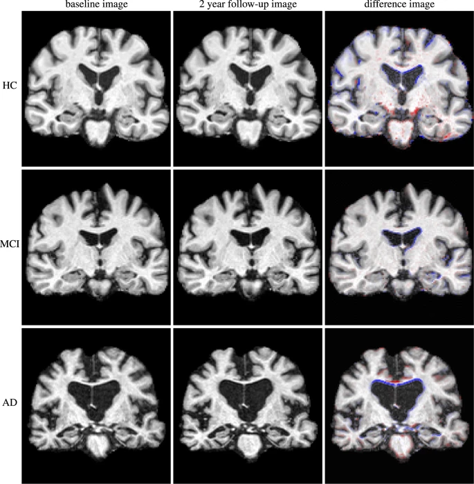
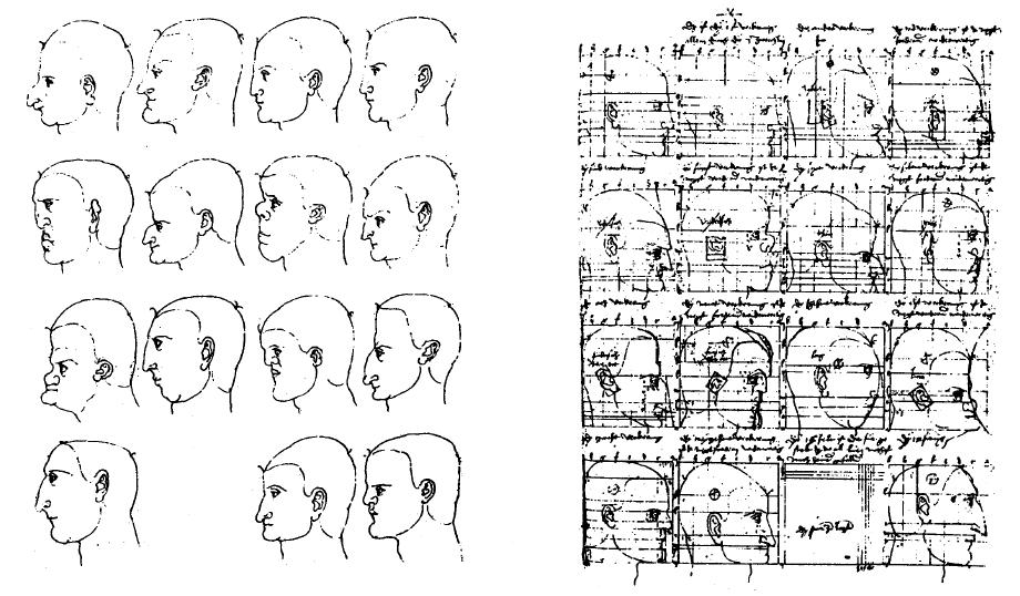
Fig. 22 This figure illustrates morphological differences between individuals with different clinical profiles: without cognitive impairment (top), mild cognitive impairment (middle), Alzheimer-type dementia (bottom). Furthermore, it is also possible to observe longitudinal differences within the same individual (from left to right, initial visit, follow-up after two years, difference between the two images). Figure taken from [Ledig et al., 2018], under CC-BY license.¶

As shown in the figure above, MRI morphological studies make it possible to compare individuals and groups. Such comparisons can tell us about the effect of age, or even the effect of injury or disease on brain shape.

Volumetry¶

Manual segmentation¶

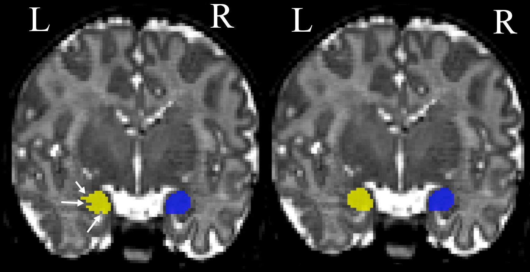
Fig. 23 This figure illustrates a manual amygdala segmentation protocol. Coronal view of a manual segmentation of the left (yellow) and right (blue) tonsil before (left) and after (right) making corrections in the coronal plane. Figure taken from [Hashempour et al., 2019], under CC-BY license.¶

Manual volumetry involves visually delineating a particular brain area, such as the hippocampus or the amygdala (see Fig. 23). This approach is time consuming, as the outline of the structures of interest must be drawn by hand on each MRI slice. We first start by segmenting a structure in a first cutting plane (for example, in the axial plane), then we will have to correct this segmentation in the other planes (for example, in the sagittal plane, then in the coronal plane).

For a reminder about the different types of brain slices, please refer to Chapter 1: Brain Maps.

In order to determine where a brain region is located, this type of approach also requires a segmentation protocol with clear anatomical criteria. For some structures, such as the hippocampus, there are detailed protocols (eg: [Wisse et al., 2017]). But for other regions, such as visual areas (V1, V2, etc.), it is necessary to carry out functional experiments in order to be able to delimit them. Indeed, in the latter case, the anatomical delimitations are not always available or well established.

A rigorous segmentation protocol is necessary to obtain a good level of concordance of the results between different researchers (inter-rater agreement). Some protocols also offer a certification process, which offers a guarantee that the person performing the segmentation applies the protocol correctly.

Automatic segmentation¶

%matplotlib inline


# Download the Harvard-Oxford atlas
from nilearn import datasets

# Ignore warnings
import warnings
warnings.filterwarnings("ignore")

atlas = datasets.fetch_atlas_harvard_oxford('cort-maxprob-thr25-2mm').maps
mni = datasets.fetch_icbm152_2009()

# Visualize the atlas
import matplotlib.pyplot as plt
from myst_nb import glue
from nilearn.plotting import plot_roi, view_img

atlas_fig = plt.figure(figsize=(12, 4))
plot_roi(atlas,
    bg_img=mni.t1,
    axes=atlas_fig.gca(),
    title="Harvard-Oxford Atlas",
    cut_coords=(8, -4, 9),
    colorbar=True,
    cmap='Dark2')

glue("harvard-oxford-fig", atlas_fig, display=False)

atlas_fig_int = view_img(atlas,
    title="Harvard-Oxford Atlas",
    cut_coords=(8, -4, 9),
    colorbar=True, symmetric_cmap=False, 
    cmap='Dark2')

glue("harvard-oxford-fig_int", atlas_fig_int, display=False)

interactive

Fig. 24 An example of an atlas of anatomical regions: the Harvard-Oxford Atlas. This figure is generated by python code using the nilearn library from a public dataset through the function fetch_atlas_harvard_oxford (Nilearn, section 9.2.1: Basic Atlas plotting) [Desikan et al., 2006, Frazier et al., 2005, Goldstein et al., 2007, Makris et al., 2006] (click on + to see the code).¶

static

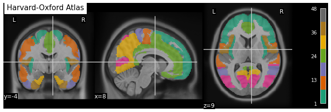
Fig. 25 An example of an atlas of anatomical regions: the Harvard-Oxford Atlas. This figure is generated by python code using the nilearn library from a public dataset through the function fetch_atlas_harvard_oxford (Nilearn, section 9.2.1: Basic Atlas plotting) [Desikan et al., 2006, Frazier et al., 2005, Goldstein et al., 2007, Makris et al., 2006] (click on + to see the code).¶

In order to automate the segmentation work, it is possible to use an atlas, ie a segmentation already carried out by a team of researchers. To do this, they constructed a map of the regions of interest inside a reference space, also called stereotactic space. There are a variety of atlases based on different anatomical or functional criteria, so it is important to choose the right atlas according to the structures studied. In order to adjust the atlas to the data of a participant, the structural images of the latter are first registered in an automated way to the stereotaxic space reference. This transformation then makes it possible to adapt the atlas to the anatomy of each participant.

Registration

In order to apply an atlas of brain regions to an individual MRI, or more generally to match two brain images, it is necessary to register this MRI on the stereotactic space that was used to establish the regions. This mathematical process will seek to deform the individual image in order to adjust it to the stereotactic space. This transformation can be affine (including in particular translation, rotation and scaling) or non-linear (movement in any direction in space). The objective of the registration is to increase the level of similarity between the images, but it is also important that the deformations are continuous. In other words, adjacent places in the unregistered images must still be adjacent after registration. The images below illustrate the effect of different types of registration. They are taken from the slicer software documentation , under CC-Attributions Share Alike license.

Fig. 26 Raw images: two scans of the same participant, taken during two different acquisition sessions.¶

../../../_images/registration_slicer_affine.gif

Fig. 27 Images registered by an affine transformation process only.¶

../../../_images/registration_slicer_nonlinear.gif

Fig. 28 Images registered by an affine transformation followed by a non-linear transformation.¶

../../../_images/registration_slicer_nonlinear_only.gif

Fig. 29 Visualization of the effects of non-linear registration only.¶

# This code retrieves T1 MRI data
# and generates an image in three planes of cuts

# Ignore warnings
import warnings
warnings.filterwarnings("ignore")

# Download an anatomical image (MNI152 template)
from nilearn.datasets import fetch_icbm152_2009
mni = fetch_icbm152_2009()

# Visualize one volume
import matplotlib.pyplot as plt
from myst_nb import glue
from nilearn.plotting import plot_anat

fig = plt.figure(figsize=(12, 4))
plot_anat(
  mni.t1,
  axes=fig.gca(),
  cut_coords=[-17, 0, 17],
  title='MNI152 stereotatic space'
)
glue("mni-template-fig", fig, display=False)

Stereotatic space

In order to define a reference anatomy, researchers generally use an “average” brain. To achieve this, the brains of several dozen individuals are aligned with each other, then averaged until a single image is obtained. If the registration worked well, as in the case of the MNI152 atlas below, the details of the neuroanatomy are preserved on average.

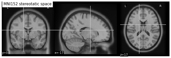
Fig. 30 Stereotaxic space of the Montreal Neurological Institute (MNI). This reference space was obtained by averaging the brain images of 152 subjects after carrying out an iterative non-linear registration [Fonov et al., 2011].¶

Statistical analyzes¶

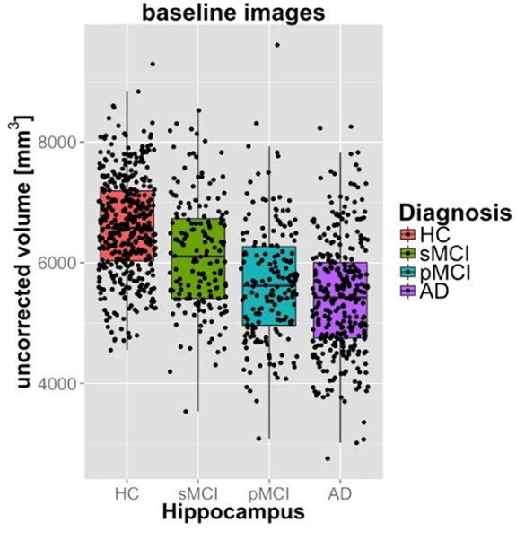
Fig. 31 This figure illustrates the differences in hippocampal volume between cognitively healthy (HC) participants, participants with stable (sMCI) or progressive (pMCI) mild cognitive impairment, and patients with Alzheimer-type dementia (AD), in the ADNI cohort. The more severe the clinical symptoms, the greater the likelihood of Alzheimer's disease, and the more severe the stage of the disease. Hippocampal atrophy is clear in patients with the most severe symptoms. Figure taken from [Ledig et al., 2018], under CC-BY license.¶

In order to carry out the statistical analyses, the volume of each segmented structure is first extracted (in \(mm^3\)). We can then statistically compare the average volume between two groups, for example, or even test the association between volume and another variable, such as age. In the example of Fig. 31, we compare the volume of the hippocampus between different clinical groups with different levels of risk for Alzheimer's disease.

Quality control¶

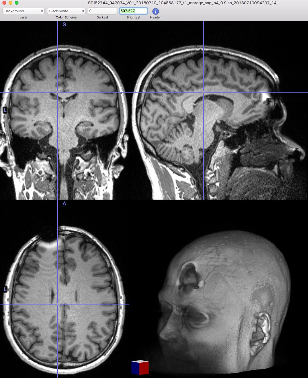
Fig. 32 The presence of metal or defective elements in the scanner can cause artefacts and distortions in the images which do not reflect the real morphology of the head. Figure of unknown origin, possibly under reserved rights.¶

It is possible to obtain aberrant results in volumetry, either because of the presence of errors in the linear and/or non-linear registration steps (Fig. 33), or because of artifacts during data acquisition (presence of metallic objects, etc. Fig. 32). It is important to perform quality control to eliminate unusable images before proceeding with statistical analyses. Retaining the latter could have significant impacts on the results as well as on the conclusions drawn.

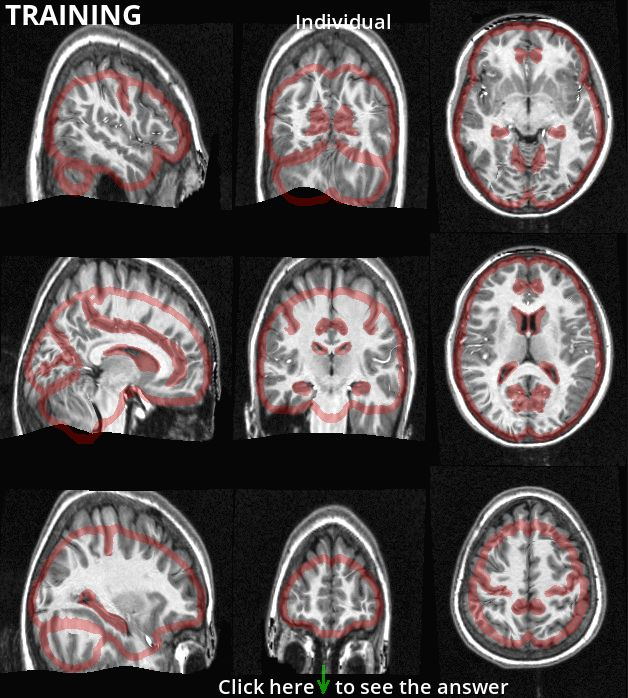
Fig. 33 Registration can sometimes fail dramatically. Here, the red shape indicates the expected outline of the brain and certain anatomical landmarks. The registered individual MRI is not at all aligned with the expected markers. Figure by P. Bellec, licensed under CC-BY.¶

VBM¶

Voxel-based morphometry (voxel-based morphometry or VBM) aims to measure the volume of gray matter located immediately around a given voxel. This approach is therefore not limited by the need to have clear pre-established boundaries between different brain structures.

Gray matter density¶

When one generates a volume measurement for all the voxels of the brain using this kind of technique, one obtains a 3D map of the density of the gray matter. The main advantages of this approach are its automated and systematic aspects. The presence of a person only becomes necessary to check that the procedure has worked correctly: this is the quality control stage (or QC, for “quality control”). We will also test the morphology of the brain through all of the gray matter. On the other hand, this technique also has a significant drawback. Indeed, the large number of measurements generated poses a problem of multiple comparisons when the time comes to perform statistical analyzes (see Chapter 9: Statistical Maps).

Segmentation¶

An important step in VBM is segmentation. This analysis aims to categorize the types of brain tissue into different classes containing gray matter, white matter, and cerebrospinal fluid, among others. A brain mask is usually extracted to exclude the meninges as well as the skull. We will generally include other types of tissue as well, such as fat. A segmentation algorithm will then examine the distribution of gray levels in the image (for example, in a T1-weighted image) and estimate for each voxel the proportion of the voxel that contains a given type of tissue. This proportion is often called the partial volume effect. A voxel can for example be assigned to 80% gray matter and 20% cerebrospinal fluid. The resulting gray level could then give a misleading indication of its actual content.

# Import necessary libraries
import matplotlib.pyplot as plt
import numpy as np
from myst_nb import glue
import seaborn as sns

# Ignore warnings
import warnings
warnings.filterwarnings("ignore")

# Download an anatomical scan (MNI152 template)
from nilearn import datasets
mni = datasets.fetch_icbm152_2009()

# Initialize the figure
fig = plt.figure(figsize=(20, 20))

from nilearn.plotting import plot_stat_map, view_img
from nilearn.image import math_img
from nilearn.input_data import NiftiMasker

thresh = 0.8
coords = [-5, 5, -25]

# Full brain
ax_plot = plt.subplot2grid((4, 3), (0, 0), colspan=1)
mask_brain = math_img(f"img>{thresh}", img=mni.mask)
val_brain = NiftiMasker(mask_img=mask_brain).fit_transform(mni.t1)
ax = sns.distplot(val_brain, norm_hist=False)
ax.set_xlim(left=0, right=100)
ax_plot = plt.subplot2grid((4, 3), (0, 1), colspan=2)
plot_stat_map(mni.mask,
              bg_img=mni.t1,
              cut_coords=coords,
              axes=ax_plot, 
              black_bg=True, colorbar=True,
              title='Brain - all'
              )

# Gray matter
ax_plot = plt.subplot2grid((4, 3), (1, 0), colspan=1)
mask_gm = math_img(f"img>{thresh}", img=mni.gm)
val_gm = NiftiMasker(mask_img=mask_gm).fit_transform(mni.t1)
ax = sns.distplot(val_gm, norm_hist=False)
ax.set_xlim(left=0, right=100)
ax_plot = plt.subplot2grid((4, 3), (1, 1), colspan=2)
plot_stat_map(mni.gm,
              bg_img=mni.t1,
              cut_coords=coords,
              axes=ax_plot,
              black_bg=True,
              title='Brain - gray matter'
              )

# White matter
ax_plot = plt.subplot2grid((4, 3), (2, 0), colspan=1)
mask_wm = math_img(f"img>{thresh}", img=mni.wm)
val_wm = NiftiMasker(mask_img=mask_wm).fit_transform(mni.t1)
ax = sns.distplot(val_wm, norm_hist=False)
ax.set_xlim(left=0, right=100)
ax_plot = plt.subplot2grid((4, 3), (2, 1), colspan=2)
plot_stat_map(mni.wm,
              bg_img=mni.t1,
              cut_coords=coords,
              axes=ax_plot,
              black_bg=True,
              title='Brain - white matter'
              )

# CSF
ax_plot = plt.subplot2grid((4, 3), (3, 0), colspan=1)
mask_csf = math_img(f"img>{thresh}", img=mni.csf)
val_csf = NiftiMasker(mask_img=mask_csf).fit_transform(mni.t1)
ax = sns.distplot(val_csf, axlabel="image intensity", norm_hist=False)
ax.set_xlim(left=0, right=100)
ax_plot = plt.subplot2grid((4, 3), (3, 1), colspan=2)
plot_stat_map(mni.csf,
              bg_img=mni.t1,
              cut_coords=coords,
              axes=ax_plot,
              black_bg=True,
              title='Brain - cerebrospinal fluid'
              )

# from myst_nb import glue
glue("mni-segmentation-fig", fig, display=False)

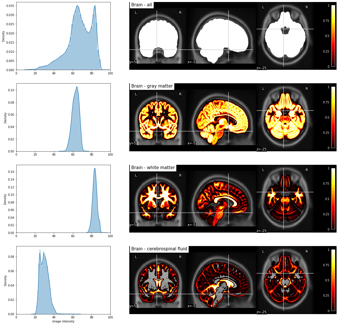
Fig. 34 Probabilistic segmentation of major tissue types and distribution of T1-weighted values in "pure" voxels (probability greater than 80% for a given tissue type). The T1-weighted image as well as the segmentations correspond to the MNI152 stereotaxic space [Fonov et al., 2011].¶

Partial volume effect

It is possible that the automatic segmentation returns to us for certain non-desired tissues values similar to those of the gray matter on the image resulting from this step. Indeed, it is possible that voxels located directly on the junction between a white zone and a black zone (for example, on a wall of white matter which would border a ventricle) have as a resulting value rather similar to gray associated with gray matter (average value between white and black). This kind of black and white blending effect is called partial volume (part of the voxel volume is white while the other part is black).

Smoothing¶

The next step is spatial smoothing. This consists of adding a filter to the image that will make it more blurred. In practice, smoothing replaces the value associated with each voxel by a weighted average of its neighbors. As it is a weighted average, the original value of the voxel is the one that will have the greatest weight, but the values of the voxels located directly around it will also affect it greatly. The value of the weights follows the profile of a 3D Gaussian distribution (the farther a neighboring voxel is from the voxel of interest, the less it will affect the value). It is necessary to perform this step in order to obtain gray matter density values for areas that exceed the single voxel, but instead represent the volume of a small region, centered on the voxel. The size of the region is controlled by a full width at half maximum, or FWHM parameter, which is measured in millimeters. The larger the FWHM value, the larger the radius of the neighborhood containing the voxels which will impact the smoothing value of the voxel (see Fig. 35).

# Import necessary libraries
import matplotlib.pyplot as plt
import numpy as np
from myst_nb import glue
import seaborn as sns

# Ignore warnings
import warnings
warnings.filterwarnings("ignore")

# Download an anatomical image (template MNI152)
from nilearn import datasets
mni = datasets.fetch_icbm152_2009()

# Initialize a figure
fig = plt.figure(figsize=(15, 15))

from nilearn.plotting import plot_anat
from nilearn.image import math_img
from nilearn.input_data import NiftiMasker
from nilearn.image import smooth_img

list_fwhm = (0, 5, 8, 10)
n_fwhm = len(list_fwhm)
coords = [-5, 5, -25]

for num, fwhm in enumerate(list_fwhm):
    ax_plot = plt.subplot2grid((n_fwhm, 1), (num, 0), colspan=1)
    vol = smooth_img(mni.gm, fwhm)
    plot_anat(vol,
              cut_coords=coords,
              axes=ax_plot,
              black_bg=True,
              title=f'FWHM={fwhm}',
              vmax=1)

from myst_nb import glue
glue("smoothing-fig", fig, display=False)

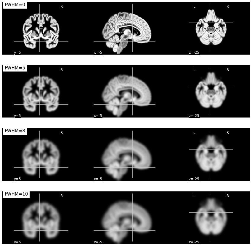
Fig. 35 Illustration of the impact of smoothing on a gray matter density map in VBM. As the FWHM parameter increases, the density measurement represents an increasingly larger region surrounding the voxel. This figure is generated by python code using the nilearn library from a public dataset called MNI152 2009 template [Fonov et al., 2011] (click on + to see the code).¶

Statistical analyzes¶

import numpy as np
import matplotlib.pyplot as plt
from nilearn import datasets
from nilearn.input_data import NiftiMasker
from nilearn.image import get_data
from nilearn.plotting import plot_stat_map, view_img 

n_subjects = 100  # more subjects requires more memory

# Load data
oasis_dataset = datasets.fetch_oasis_vbm(n_subjects=n_subjects)
gray_matter_map_filenames = oasis_dataset.gray_matter_maps
age = oasis_dataset.ext_vars['age'].astype(float)

# Prepare mask
nifti_masker = NiftiMasker(
    standardize=False,
    smoothing_fwhm=2,
    memory='nilearn_cache')  # cache options

# Normalize data
gm_maps_masked = nifti_masker.fit_transform(gray_matter_map_filenames)

from sklearn.feature_selection import VarianceThreshold
variance_threshold = VarianceThreshold(threshold=.01)

gm_maps_thresholded = variance_threshold.fit_transform(gm_maps_masked)
gm_maps_masked = variance_threshold.inverse_transform(gm_maps_thresholded)
data = variance_threshold.fit_transform(gm_maps_masked)

# Massively univariate regression model
from nilearn.mass_univariate import permuted_ols
neg_log_pvals, t_scores_original_data, _ = permuted_ols(
    age, data,  # + intercept as a covariate by default
    n_perm=20,  # 1,000 in the interest of time; 10000 would be better
    verbose=1, # display progress bar
    n_jobs=1)  # can be changed to use more CPUs
signed_neg_log_pvals = neg_log_pvals * np.sign(t_scores_original_data)
signed_neg_log_pvals_unmasked = nifti_masker.inverse_transform(
    variance_threshold.inverse_transform(signed_neg_log_pvals))

# Visualize result
threshold = -np.log10(0.1)  # 10% corrected

fig = plt.figure(figsize=(25, 8), facecolor='k')
bg_filename = gray_matter_map_filenames[0]
cut_coords = [0, 0, 0]
stat_exp = plot_stat_map(signed_neg_log_pvals_unmasked, bg_img=bg_filename,
                        threshold=threshold, cmap=plt.cm.RdBu_r,
                        cut_coords=cut_coords, figure=fig)
title = ('Negative $\\log_{10}$ p-values'
         '\n(Non-parametric + max-type correction)')
stat_exp.title(title, y=1.2, size=50)
plt.show()

from myst_nb import glue
glue("vbm-fig", fig, display=False)


stat_exp_int = view_img(signed_neg_log_pvals_unmasked, bg_img=bg_filename,
                        threshold=threshold, cmap=plt.cm.RdBu_r,
                        colorbar=True, title='Negative log10 p-values'
                                             '\n(Non-parametric + max-type correction)')

glue("vbm-fig_int", stat_exp_int, display=False)

interactive

Fig. 36 Linear regression in VBM. We are testing here the effect of age on a group of participants (N=50) from the OASIS database. The \(-\log_{10}(p)\) significance of the age effect is superimposed on a gray matter density image. This figure is adapted from a Nilearn tutorial.¶

static

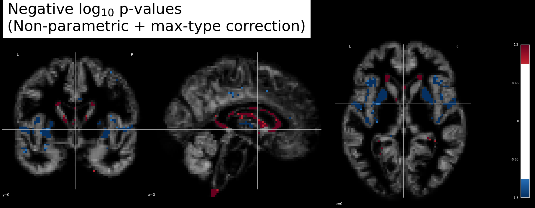
Fig. 37 Linear regression in VBM. We are testing here the effect of age on a group of participants (N=50) from the OASIS database. The \(-\log_{10}(p)\) significance of the age effect is superimposed on a gray matter density image. This figure is adapted from a Nilearn tutorial.¶

In order to be able to compare gray matter density values between participants, we use the same non-linear registration-tip> procedure as for automatic volumetry. Unlike manual volumetry, where each volume under study is delimited so as to represent the same structure of interest, the registration used in VBM is not linked to a particular structure. Once the density maps have been readjusted in the reference stereotactic space, statistical tests can be carried out at each voxel. In the example above, we test the effect of age on gray matter. It is generally this kind of image that will subsequently be inserted into scientific publications.

Quality control¶

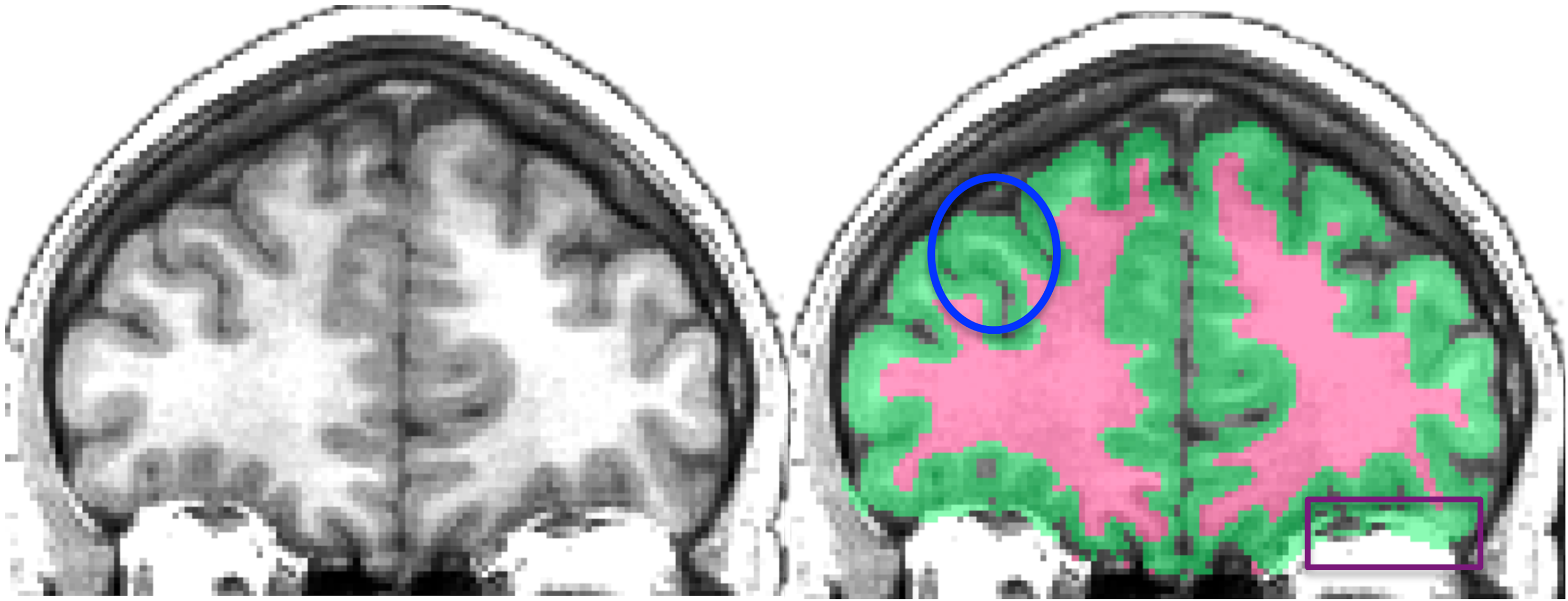
../../../_images/segmentation-error-volume-fig.png

Fig. 38 Left image: Individual T1-weighted MRI. Right image: gray matter and white matter classification generated by the software ANTS. Note how white matter near the gyrus is erroneously classified as gray matter. CC Attribution licensed image from [Klein et al., 2017].¶

As with any automated operation, there is always the possibility of error in VBM. It is therefore necessary to provide a quality control step in order to ensure that there have been no aberrations which have been introduced into the processing steps. We have already discussed artefacts in the data as well as registration problems. The VBM is also very sensitive to errors in the segmentation step. It is therefore possible to lose certain structures for which the contrast between the white matter and the gray matter is not significant enough for the algorithm to succeed in classifying them effectively. For this kind of structure, it is important to add a priori (additional rules or conditions) in order not to lose them. It is also possible to correct this part of the segmentation manually or to exclude the data of certain participants.

Surface analyses¶

Surface extraction¶

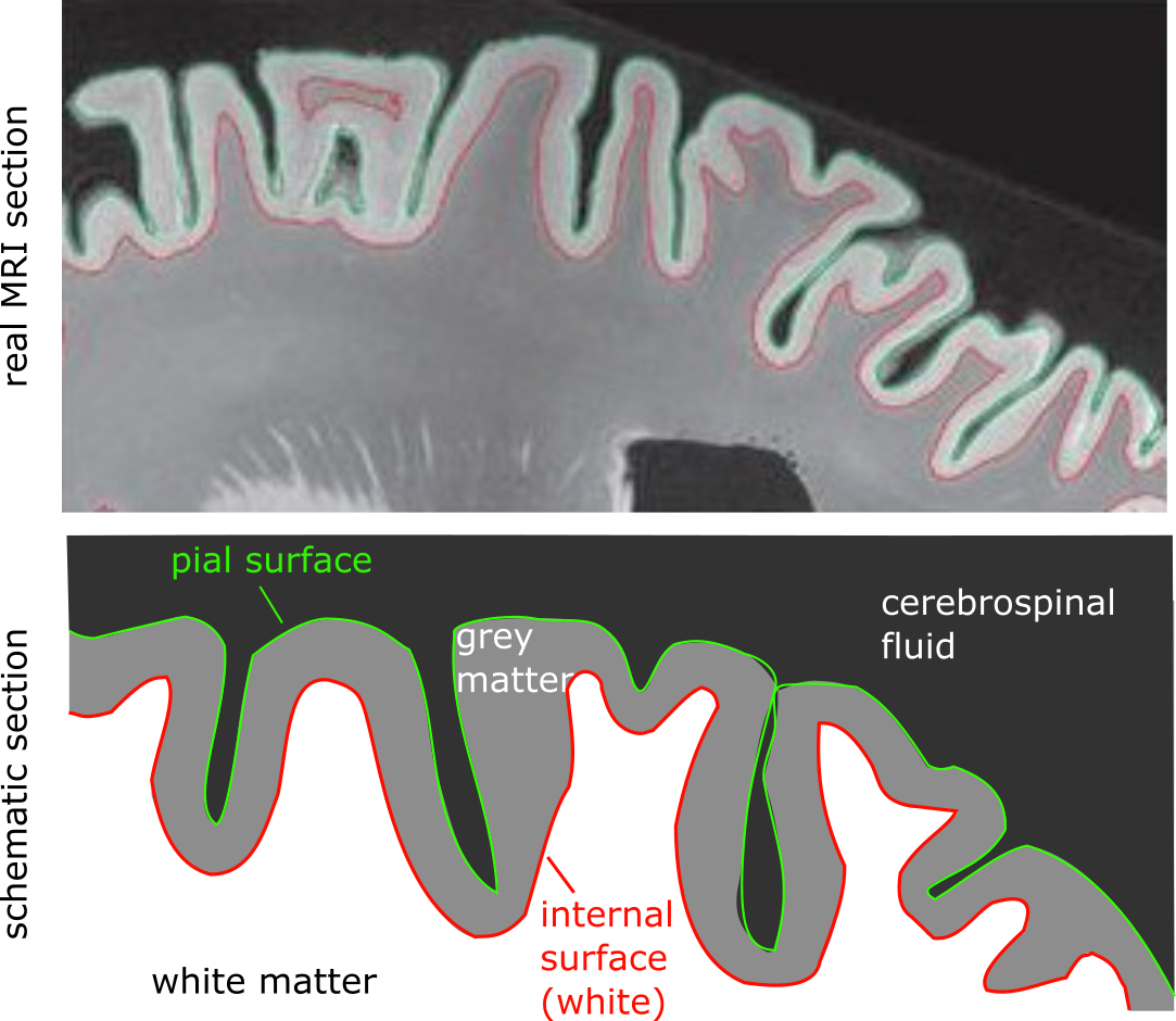
Fig. 39 Illustration of the position of the pial surface and the inner surface. Top: T1-weighted MRI slice with automatically estimated areas. Bottom: schematic illustration of the surfaces. Figure adapted by P. Bellec from figures in the article by [Klein et al., 2017] under CC-BY license.¶

Cortical surface analyzes differ from the previously outlined morphometry techniques in that they exploit the ribbon that gray matter forms by extending across the surface of white matter. In addition to the segmentation and registration steps that we saw previously, we will use here an algorithm that will detect the pial surface, at the border between the gray matter and the cerebrospinal fluid, and the pial surface, at the border between the gray matter and the cerebrospinal fluid, and the pial surface interior (also called white surface), at the border between white matter and gray matter. It will also be necessary, as for VBM, to extract a mask from the brain by eliminating structures that do not belong to the cortex (cranial box, adipose tissue, meninges, cerebrospinal fluid, etc.). This kind of analysis produces surfaces that can be viewed as 3D objects, resulting in magnificent interactive visualizations.

Balloon growth

To estimate the position of the pial and inner surfaces, a virtual balloon is placed in the center of each of the hemispheres of the brain. We then model physical constraints at the boundary between white matter and gray matter (internal surface). We then proceed to "inflate" this balloon until it matches the border of the internal surface as best as possible (until the balloon is inflated and occupies all the space in the cavity and that it matches all the curves of the wall). It is also possible to do the reverse procedure. We could indeed generate a virtual balloon around each of the hemispheres and "deflate" them until they match the contours of the borders delimited by the physical constraints. When one of the borders (internal surface or pial surface) is delimited, it is possible to continue the inflation/deflation procedure in order to obtain the second surface.

Attention

Surface extraction techniques such as those proposed by the FreeSurfer software are costly in terms of computational resources. Generating a surface from a structural MRI can take up to 10 hours on a standard computer.

Thickness, area and volume¶

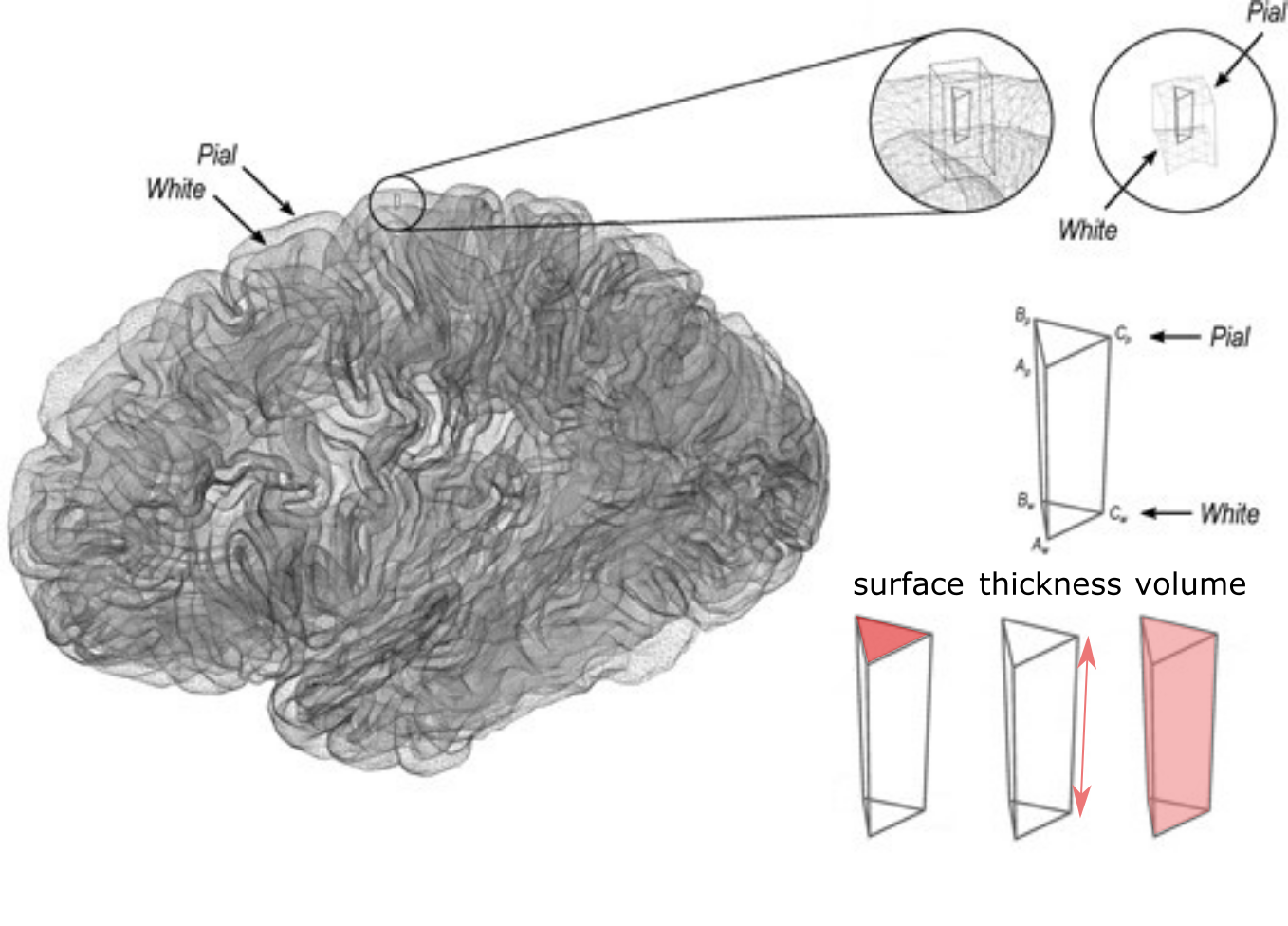
Fig. 40 Illustration of area, thickness and volume measurements of the cortex. Figure adapted by P. Bellec from figures in the article by [Winkler et al., 2018] under CC-BY license.¶

The reconstruction of the geometry of the surface will make it possible to decompose the volume of the gray matter into a local thickness, and a local surface. These two properties can now be studied separately, unlike what is possible with a VBM analysis, and have been shown to be independently linked to different neurological and psychiatric conditions. To do this, instead of analyzing the content of volume units (voxels), as was the case for VBM, we will use here the analysis of the content of surface units: the vertices .

Attention

Who says cortical surface, also implies that the subcortical structures are left aside. For structures buried in the cranium, such as the thalami and basal ganglia, surface analysis must be combined with automatic volumetry (for subcortical structures).

Statistical analyses¶

from nilearn import datasets
fsaverage = datasets.fetch_surf_fsaverage()

from nilearn.plotting import plot_surf_stat_map, view_img_on_surf
from nilearn.surface import vol_to_surf
fig = plt.figure(figsize=(10, 8))

texture = vol_to_surf(signed_neg_log_pvals_unmasked, fsaverage.pial_right)

plot_surf_stat_map(fsaverage.white_right, texture, hemi='right', view='lateral',
                            title='Right hemisphere white surface', colorbar=True,
                            threshold=0.5, bg_map=fsaverage.sulc_right,
                            figure=fig)

# from myst_nb import glue
glue("surf_stat_fig", fig, display=False)


surf_exp = view_img_on_surf(signed_neg_log_pvals_unmasked, fsaverage, 
                            title='White surface', colorbar=True,
                            threshold=0.5)

glue("surf_stat_fig_int", surf_exp, display=False)

interactive

Fig. 41 Projection of the statistical map presented in vbm-fig onto the cortical surface space fsaverage. This figure is adapted from a Nilearn tutorial.¶

interactive

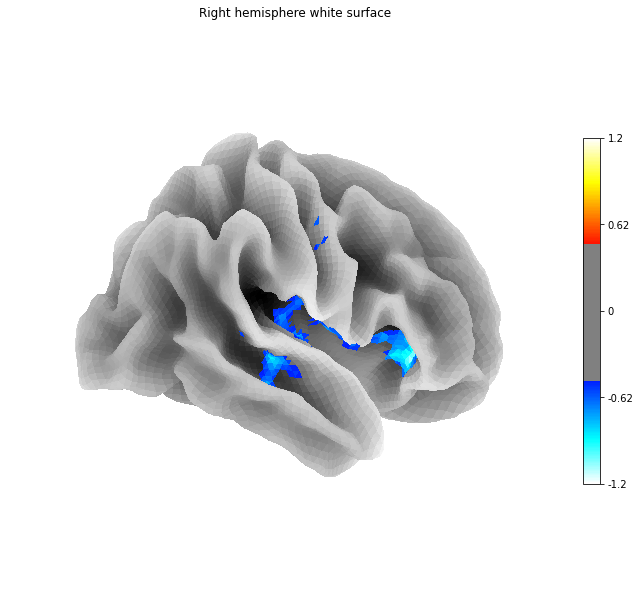
Fig. 42 Projection of the statistical map presented in vbm-fig onto the cortical surface space fsaverage. This figure is adapted from a Nilearn tutorial.¶

Statistical analyzes work exactly the same way for surface analyzes as for VBM. But instead of doing a statistical test at the level of each of the voxels (as in VBM), we now do a test for each of the vertices (surface).

Quality control¶

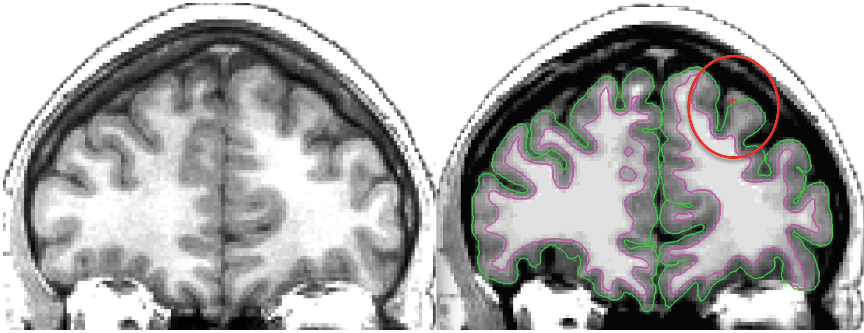
../../../_images/segmentation-error-surface-fig.png

Fig. 43 Left image: Individual T1-weighted MRI. Right image: Automated surface extraction. Note that the pial surface does not properly follow the interface between gray matter and cerebrospinal fluid where indicated. CC Attribution licensed image from [Klein et al., 2017].¶

The surface extraction technique is not robust to partial volume effects. One could indeed have a surface which does not go to the bottom of a sulcus, or when the gyri are very close together, which does not even enter inside the sulcus. The result of these two types of error, which are possible both at the level of the pial surface and the internal surface, will be a strong localized overestimation of the cortical thickness. This is why it is desirable to carry out frequent quality checks on all images and to correct segmentation errors by hand, or else to exclude the data of certain participants.

Conclusion¶

This chapter of the course introduced you to the different families of computational morphology techniques that can be used with data acquired in anatomical magnetic resonance imaging. Several key image analysis techniques were discussed and some statistical models started to be introduced.

References¶

1(1,2): Rahul S. Desikan, Florent Ségonne, Bruce Fischl, Brian T. Quinn, Bradford C. Dickerson, Deborah Blacker, Randy L. Buckner, Anders M. Dale, R. Paul Maguire, Bradley T. Hyman, Marilyn S. Albert, and Ronald J. Killiany. An automated labeling system for subdividing the human cerebral cortex on MRI scans into gyral based regions of interest. NeuroImage, 31(3):968–980, July 2006. URL: https://www.sciencedirect.com/science/article/pii/S1053811906000437 (visited on 2022-04-01), doi:10.1016/j.neuroimage.2006.01.021.
2(1,2,3): Vladimir Fonov, Alan C. Evans, Kelly Botteron, C. Robert Almli, Robert C. McKinstry, and D. Louis Collins. Unbiased average age-appropriate atlases for pediatric studies. NeuroImage, 54(1):313–327, January 2011. URL: https://www.sciencedirect.com/science/article/pii/S1053811910010062 (visited on 2022-04-01), doi:10.1016/j.neuroimage.2010.07.033.
3(1,2): Jean A. Frazier, Sufen Chiu, Janis L. Breeze, Nikos Makris, Nicholas Lange, David N. Kennedy, Martha R. Herbert, Eileen K. Bent, Vamsi K. Koneru, Megan E. Dieterich, Steven M. Hodge, Scott L. Rauch, P. Ellen Grant, Bruce M. Cohen, Larry J. Seidman, Verne S. Caviness, and Joseph Biederman. Structural Brain Magnetic Resonance Imaging of Limbic and Thalamic Volumes in Pediatric Bipolar Disorder. American Journal of Psychiatry, 162(7):1256–1265, July 2005. Publisher: American Psychiatric Publishing. URL: https://ajp.psychiatryonline.org/doi/full/10.1176/appi.ajp.162.7.1256 (visited on 2022-04-01), doi:10.1176/appi.ajp.162.7.1256.
4(1,2): Jill M. Goldstein, Larry J. Seidman, Nikos Makris, Todd Ahern, Liam M. O’Brien, Verne S. Caviness, David N. Kennedy, Stephen V. Faraone, and Ming T. Tsuang. Hypothalamic Abnormalities in Schizophrenia: Sex Effects and Genetic Vulnerability. Biological Psychiatry, 61(8):935–945, April 2007. Publisher: Elsevier. URL: https://www.biologicalpsychiatryjournal.com/article/S0006-3223(06)00819-5/fulltext (visited on 2022-04-01), doi:10.1016/j.biopsych.2006.06.027.
5: Niloofar Hashempour, Jetro J. Tuulari, Harri Merisaari, Kristian Lidauer, Iiris Luukkonen, Jani Saunavaara, Riitta Parkkola, Tuire Lähdesmäki, Satu J. Lehtola, Maria Keskinen, John D. Lewis, Noora M. Scheinin, Linnea Karlsson, and Hasse Karlsson. A Novel Approach for Manual Segmentation of the Amygdala and Hippocampus in Neonate MRI. Frontiers in Neuroscience, 2019. URL: https://www.frontiersin.org/article/10.3389/fnins.2019.01025 (visited on 2022-04-01).
6(1,2,3): Arno Klein, Satrajit S. Ghosh, Forrest S. Bao, Joachim Giard, Yrjö Häme, Eliezer Stavsky, Noah Lee, Brian Rossa, Martin Reuter, Elias Chaibub Neto, and Anisha Keshavan. Mindboggling morphometry of human brains. PLOS Computational Biology, 13(2):e1005350, February 2017. Publisher: Public Library of Science. URL: https://journals.plos.org/ploscompbiol/article?id=10.1371/journal.pcbi.1005350 (visited on 2022-04-01), doi:10.1371/journal.pcbi.1005350.
7(1,2): Christian Ledig, Andreas Schuh, Ricardo Guerrero, Rolf A. Heckemann, and Daniel Rueckert. Structural brain imaging in Alzheimer’s disease and mild cognitive impairment: biomarker analysis and shared morphometry database. Scientific Reports, 8(1):11258, July 2018. Number: 1 Publisher: Nature Publishing Group. URL: https://www.nature.com/articles/s41598-018-29295-9 (visited on 2022-04-01), doi:10.1038/s41598-018-29295-9.
8(1,2): Nikos Makris, Jill M. Goldstein, David Kennedy, Steven M. Hodge, Verne S. Caviness, Stephen V. Faraone, Ming T. Tsuang, and Larry J. Seidman. Decreased volume of left and total anterior insular lobule in schizophrenia. Schizophrenia Research, 83(2):155–171, April 2006. URL: https://www.sciencedirect.com/science/article/pii/S0920996405004998 (visited on 2022-04-01), doi:10.1016/j.schres.2005.11.020.
9: Anderson M Winkler, Douglas N Greve, Knut J Bjuland, Thomas E Nichols, Mert R Sabuncu, Asta K Håberg, Jon Skranes, and Lars M Rimol. Joint Analysis of Cortical Area and Thickness as a Replacement for the Analysis of the Volume of the Cerebral Cortex. Cerebral Cortex, 28(2):738–749, February 2018. URL: https://doi.org/10.1093/cercor/bhx308 (visited on 2022-04-01), doi:10.1093/cercor/bhx308.
10: Laura E.M. Wisse, Ana M. Daugherty, Rosanna K. Olsen, David Berron, Valerie A. Carr, Craig E.L. Stark, Robert S.C. Amaral, Katrin Amunts, Jean C. Augustinack, Andrew R. Bender, Jeffrey D. Bernstein, Marina Boccardi, Martina Bocchetta, Alison Burggren, M. Mallar Chakravarty, Marie Chupin, Arne Ekstrom, Robin de Flores, Ricardo Insausti, Prabesh Kanel, Olga Kedo, Kristen M. Kennedy, Geoffrey A. Kerchner, Karen F. LaRocque, Xiuwen Liu, Anne Maass, Nicolai Malykhin, Susanne G. Mueller, Noa Ofen, Daniela J. Palombo, Mansi B. Parekh, John B. Pluta, Jens C. Pruessner, Naftali Raz, Karen M. Rodrigue, Dorothee Schoemaker, Andrea T. Shafer, Trevor A. Steve, Nanthia Suthana, Lei Wang, Julie L. Winterburn, Michael A. Yassa, Paul A. Yushkevich, Renaud la Joie, and for the Hippocampal Subfields Group. A harmonized segmentation protocol for hippocampal and parahippocampal subregions: Why do we need one and what are the key goals? Hippocampus, 27(1):3–11, 2017. _eprint: https://onlinelibrary.wiley.com/doi/pdf/10.1002/hipo.22671. URL: https://onlinelibrary.wiley.com/doi/abs/10.1002/hipo.22671 (visited on 2022-04-01), doi:10.1002/hipo.22671.

Exercices¶

Exercice 3.1

Choose the best answer and explain why. Individual T1 MRI data are…

A 3D image of a brain.
Dozens of 2D sagittal images of a brain.
Hundreds of axial, coronal and sagittal 2D images of a brain.
All of the above.

Exercice 3.2

We want to compare the mean volume of the right putamen between neurotypical participants and participants on the autism spectrum. Two alternative methods are considered for this: manual volumetry and VBM analysis. For each of these techniques, name a strength and a weakness in relation to the objectives of the study.

Exercice 3.3

For each of the following statements, specify whether the statement is true or false and explain your choice.

T1 MRI data needs to be realigned to study brain morphology at the population level.
"Raw" MRI data (before the pre-processing step) cannot be used to study morphometry.
In VBM, spatial smoothing is important, even for an individual analysis.

Exercice 3.4

For each of the following statements, specify whether the statement is true or false and explain your choice.

The movements of a research participant can create noise in a VBM map.
The presence of metal can create noise and distortions in a VBM card.
A hole in a VBM brain map necessarily means that there is a hole in the participant’s brain.

Exercice 3.5

While checking her structural data, a researcher realizes that one of her research participants has twice the normal brain volume! However, this participant’s skull appeared normal. Offer an explanation.

Exercice 3.6

We wish to make a comparison between the quantity of gray matter present at the level of the post-central sulcus and that contained in the precentral sulcus, on average, over a population. Two alternative methods are considered for this: a VBM analysis or an analysis of the cortical thickness (surface analysis). Which technique would you choose and why?

Exercice 3.7

Data from one research participant is of poor quality and gray matter segmentation is imprecise. For each of the following combinations of choices, which technique would you choose and why?

VBM vs manual volumetrics?
VBM vs surface analysis?

Exercice 3.8

We have seen in class some examples of cerebral anatomical structures. Let’s do a little review… Using the visualization window below (also accessible on this course web page), give the coordinates (x, y, or z) where you can see…

a sagittal section showing the corpus callosum.
a coronal section showing the corpus callosum.
an axial section containing ventricles.
an axial section with the central sulcus.

For a refresher on the different types of brain slices, please refer to Chapter 1: Brain Maps.

# This code retrieves T1 MRI data
# and generates an image in three planes of cuts

# Ignore warnings
import warnings
warnings.filterwarnings("ignore")

# Download an anatomical scan
from nilearn.datasets import fetch_icbm152_2009
mni = fetch_icbm152_2009()

# Visualize a cerebral volume
from nilearn.plotting import view_img

view_img(
    mni.t1,
    bg_img=None,
    black_bg=True,
    cut_coords=[-17, 0, 17],
    title='T1w image',
    cmap='gray',
    colorbar=False,
    symmetric_cmap=False
)

Exercice 3.9

To answer the questions in this exercise, first read the article Development of cortical thickness and surface area in autism spectrum disorder by Mensen et al. (published in 2017 in the journal Neuroimage: Clinical, volume 13, pages 215 at 222). It is freely available at this address. The following questions require short-text answers.

What type(s) of participant(s) were recruited in this study?
What is the main objective of the study?
What are the inclusion and exclusion criteria?
What neuroimaging technique is used? Is it a structural or functional technique?
What type of image acquisition sequence is used? List the parameters.
Does image processing include a registration step(s)? If yes, what type(s)?
Do the researchers have a quality control procedure in place? If yes, summarize this procedure.
Are the regions of interest (ROI) defined? If yes, in what way? With which atlas? How many are there?
What morphological measures are used for each region?
Which figure (or table) meets the main objective of the study?

Spring/Fall term 2022

Morphometric analyzes

Contents

Morphometric analyzes¶

Objectives 📍¶

Morphometry¶

Volumetry¶

Manual segmentation¶

Automatic segmentation¶

Statistical analyzes¶

Quality control¶

VBM¶

Gray matter density¶

Segmentation¶

Smoothing¶

Statistical analyzes¶

Quality control¶

Surface analyses¶

Surface extraction¶

Thickness, area and volume¶

Statistical analyses¶

Quality control¶

Conclusion¶

References¶

Exercices¶