%matplotlib inline

Nilearn GLM: statistical analyses of MRI in Python¶

Nilearn’s GLM/stats module allows fast and easy MRI statistical analysis.

It leverages Nibabel and other Python libraries from the Python scientific stack like Scipy, Numpy and Pandas.

In this tutorial, we’re going to explore nilearn's GLM functionality by analyzing 1) a single subject single run and 2) three subject group level example using a General Linear Model (GLM). We’re gonna use the same example dataset (ds000114) as from the nibabel and nilearn tutorials. As this is a multi run multi task dataset, we’ve to decide on a run and a task we want to analyze. Let’s go with ses-test and task-fingerfootlips, starting with a single subject sub-01.

Individual level analysis¶

Setting and inspecting the data¶

At first, we have to set and indicate the data we want to analyze. As stated above, we’re going to use the anatomical image and the preprocessed functional image of sub-01 from ses-test. The preprocessing was conducted through fmriprep.

fmri_img = '/data/ds000114/derivatives/fmriprep/sub-01/ses-test/func/sub-01_ses-test_task-fingerfootlips_space-MNI152nlin2009casym_desc-preproc_bold.nii.gz'
anat_img = '/data/ds000114/sub-01/ses-test/anat/sub-01_ses-test_T1w.nii.gz'

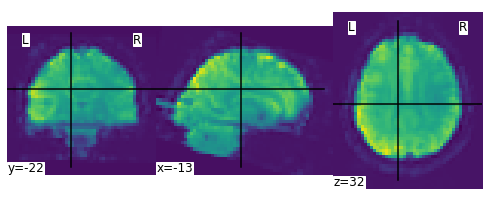
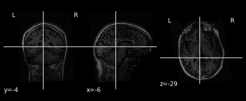
We can display the mean functional image and the subject’s anatomy:

from nilearn.image import mean_img
mean_img = mean_img(fmri_img)

from nilearn.plotting import plot_stat_map, plot_anat, plot_img, show, plot_glass_brain
plot_img(mean_img)
plot_anat(anat_img)

<nilearn.plotting.displays.OrthoSlicer at 0x7fba6a6fe8d0>

../_images/statistical_analyses_MRI_7_1.png

../_images/statistical_analyses_MRI_7_2.png

Specifying the experimental paradigm¶

We must now provide a description of the experiment, that is, define the timing of the task and rest periods. This is typically provided in an events.tsv file.

import pandas as pd
events = pd.read_table('/data/ds000114/task-fingerfootlips_events.tsv')
print(events)

    onset  duration  weight trial_type
    10      15.0       1     Finger
    40      15.0       1       Foot
    70      15.0       1       Lips
   100      15.0       1     Finger
   130      15.0       1       Foot
   160      15.0       1       Lips
   190      15.0       1     Finger
   220      15.0       1       Foot
   250      15.0       1       Lips
   280      15.0       1     Finger
  310      15.0       1       Foot
  340      15.0       1       Lips
  370      15.0       1     Finger
  400      15.0       1       Foot
  430      15.0       1       Lips

Performing the GLM analysis¶

It is now time to create and estimate a FirstLevelModel object, that will generate the design matrix using the information provided by the events object.

from nilearn.glm.first_level import FirstLevelModel

There are a lot of important parameters one needs to define within a FirstLevelModel and the majority of them will have a prominent influence on your results. Thus, make sure to check them before running your model:

FirstLevelModel?

We need the TR of the functional images, luckily we can extract that information using nibabel:

!nib-ls /data/ds000114/sub-01/ses-test/func//data/ds000114/derivatives/fmriprep/sub-01/ses-test/func/sub-01_ses-test_task-fingerfootlips_space-MNI152nlin2009casym_desc-preproc_bold.nii.gz

/data/ds000114/sub-01/ses-test/func//data/ds000114/derivatives/fmriprep/sub-01/ses-test/func/sub-01_ses-test_task-fingerfootlips_space-MNI152nlin2009casym_desc-preproc_bold.nii.gz failed

As we can see the TR is 2.5.

fmri_glm = FirstLevelModel(t_r=2.5,
                           noise_model='ar1',
                           hrf_model='spm',
                           drift_model='cosine',
                           high_pass=1./160,
                           signal_scaling=False,
                           minimize_memory=False)

Usually, we also want to include confounds computed during preprocessing (e.g., motion, global signal, etc.) as regressors of no interest. In our example, these were computed by fmriprep and can be found in derivatives/fmriprep/sub-01/func/. We can use pandas to inspect that file:

import pandas as pd
confounds = pd.read_csv('/data/ds000114/derivatives/fmriprep/sub-01/ses-test/func/sub-01_ses-test_task-fingerfootlips_bold_desc-confounds_timeseries.tsv', delimiter='\t')
confounds

	WhiteMatter	GlobalSignal	stdDVARS	non-stdDVARS	vx-wisestdDVARS	FramewiseDisplacement	tCompCor00	tCompCor01	tCompCor02	tCompCor03	...	aCompCor02	aCompCor03	aCompCor04	aCompCor05	X	Y	Z	RotX	RotY	RotZ
0	59.958244	296.705627	NaN	NaN	NaN	NaN	-0.945194	0.178691	-0.008839	0.023860	...	0.001226	-0.070598	0.040292	-0.004502	-6.811590e-03	0.000000	0.000000	0.000000	-0.000000	0.000000
1	-0.992987	-6.791035	10.967166	359.572876	15.125442	0.522051	0.095183	-0.081205	0.043344	-0.067988	...	-0.006754	0.102960	-0.020727	0.005408	-1.198610e-09	-0.035396	0.386632	0.001864	-0.000000	0.000000
2	0.121577	-8.960917	0.965478	31.654449	1.251122	0.053361	0.039534	-0.048124	0.023519	-0.009606	...	-0.006754	0.096988	-0.022278	-0.102161	0.000000e+00	-0.019626	0.383440	0.001176	-0.000000	0.000000
3	-3.207463	-15.836485	0.568300	18.632469	0.933274	0.079333	0.064448	-0.049706	0.013449	-0.031648	...	-0.036826	0.078502	0.003200	-0.112108	0.000000e+00	-0.032375	0.430492	0.001567	-0.000000	0.000000
4	-3.531865	-16.072039	0.412484	13.523833	1.089049	0.030417	0.058324	-0.050976	0.013930	-0.027509	...	-0.024400	0.069612	0.006408	-0.060869	2.562640e-10	-0.032767	0.404579	0.001485	-0.000000	0.000000
...	...	...	...	...	...	...	...	...	...	...	...	...	...	...	...	...	...	...	...	...	...
179	-1.131588	6.617327	0.796877	26.126665	0.812802	0.162573	0.001240	-0.007174	-0.044028	-0.010630	...	-0.076143	0.074762	0.004733	0.020203	-5.966000e-01	0.258395	1.762940	0.000232	0.003428	-0.013078
180	-2.441096	3.395323	0.606146	19.873285	0.689635	0.080021	0.003447	0.006033	-0.038060	0.003348	...	0.006482	0.081220	0.004589	-0.054566	-6.161150e-01	0.237964	1.772880	0.000388	0.003602	-0.013351
181	-4.028681	-0.000021	0.725305	23.780071	0.768956	0.195117	0.008511	0.018631	-0.045767	0.042005	...	0.019911	-0.027145	-0.028081	0.013844	-6.761900e-01	0.216604	1.814620	-0.000184	0.003883	-0.013937
182	-4.716608	0.375874	0.549176	18.005463	0.654098	0.085730	0.009503	0.000066	-0.031858	-0.026816	...	0.026724	0.012923	0.025031	0.012589	-6.877110e-01	0.198889	1.825820	-0.000529	0.004307	-0.013800
183	-2.884027	2.981873	0.582871	19.110176	0.675460	0.453545	0.004254	-0.009564	-0.043303	-0.052722	...	-0.014826	0.072763	0.044807	-0.027618	-5.796220e-01	0.244931	1.756250	0.000987	0.003099	-0.011926

184 rows × 24 columns

Comparable to other neuroimaging softwards, we have a timepoint x confound dataframe. However, fmriprep computes way more confounds than most of you are used to and that require a bit of reading to understand and therefore utilize properly. We therefore and for the sake of simplicity stick to the “classic” ones: WhiteMatter, GlobalSignal, FramewiseDisplacement and the motion correction parameters in translation and rotation:

import numpy as np
confounds_glm = confounds[['WhiteMatter', 'GlobalSignal', 'FramewiseDisplacement', 'X', 'Y', 'Z', 'RotX', 'RotY', 'RotZ']].replace(np.nan, 0)
confounds_glm

	WhiteMatter	GlobalSignal	FramewiseDisplacement	X	Y	Z	RotX	RotY	RotZ
0	59.958244	296.705627	0.000000	-6.811590e-03	0.000000	0.000000	0.000000	-0.000000	0.000000
1	-0.992987	-6.791035	0.522051	-1.198610e-09	-0.035396	0.386632	0.001864	-0.000000	0.000000
2	0.121577	-8.960917	0.053361	0.000000e+00	-0.019626	0.383440	0.001176	-0.000000	0.000000
3	-3.207463	-15.836485	0.079333	0.000000e+00	-0.032375	0.430492	0.001567	-0.000000	0.000000
4	-3.531865	-16.072039	0.030417	2.562640e-10	-0.032767	0.404579	0.001485	-0.000000	0.000000
...	...	...	...	...	...	...	...	...	...
179	-1.131588	6.617327	0.162573	-5.966000e-01	0.258395	1.762940	0.000232	0.003428	-0.013078
180	-2.441096	3.395323	0.080021	-6.161150e-01	0.237964	1.772880	0.000388	0.003602	-0.013351
181	-4.028681	-0.000021	0.195117	-6.761900e-01	0.216604	1.814620	-0.000184	0.003883	-0.013937
182	-4.716608	0.375874	0.085730	-6.877110e-01	0.198889	1.825820	-0.000529	0.004307	-0.013800
183	-2.884027	2.981873	0.453545	-5.796220e-01	0.244931	1.756250	0.000987	0.003099	-0.011926

184 rows × 9 columns

Now that we have specified the model, we can run it on the fMRI image

fmri_glm = fmri_glm.fit(fmri_img, events, confounds_glm)

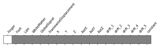
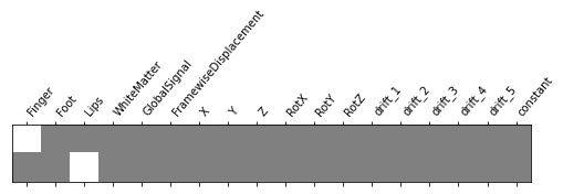
One can inspect the design matrix (rows represent time, and columns contain the predictors).

design_matrix = fmri_glm.design_matrices_[0]

Formally, we have taken the first design matrix, because the model is implictily meant to for multiple runs.

from nilearn.plotting import plot_design_matrix
plot_design_matrix(design_matrix)
import matplotlib.pyplot as plt
plt.show()

../_images/statistical_analyses_MRI_27_0.png

Save the design matrix image to disk, first creating a directory where you want to write the images:

import os
outdir = 'results'
if not os.path.exists(outdir):
    os.mkdir(outdir)

from os.path import join
plot_design_matrix(design_matrix, output_file=join(outdir, 'design_matrix.png'))

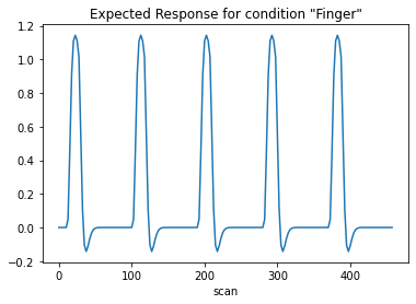
The first column contains the expected reponse profile of regions which are sensitive to the “Finger” task. Let’s plot this first column:

plt.plot(design_matrix['Finger'])
plt.xlabel('scan')
plt.title('Expected Response for condition "Finger"')
plt.show()

../_images/statistical_analyses_MRI_31_0.png

Detecting voxels with significant effects¶

To access the estimated coefficients (Betas of the GLM model), we created constrast with a single ‘1’ in each of the columns: The role of the contrast is to select some columns of the model –and potentially weight them– to study the associated statistics. So in a nutshell, a contrast is a weigted combination of the estimated effects. Here we can define canonical contrasts that just consider the two condition in isolation —let’s call them “conditions”— then a contrast that makes the difference between these conditions.

from numpy import array
conditions = {
    'active - Finger': array([1., 0., 0., 0., 0., 0., 0., 0., 0., 0., 0., 0., 0., 0., 0., 0., 0., 0.]),
    'active - Foot':   array([0., 1., 0., 0., 0., 0., 0., 0., 0., 0., 0., 0., 0., 0., 0., 0., 0., 0.]),
    'active - Lips':   array([0., 0., 1., 0., 0., 0., 0., 0., 0., 0., 0., 0., 0., 0., 0., 0., 0., 0.]),
}

Let’s look at it: plot the coefficients of the contrast, indexed by the names of the columns of the design matrix.

from nilearn.plotting import plot_contrast_matrix
plot_contrast_matrix(conditions['active - Finger'], design_matrix=design_matrix)

<AxesSubplot:label='conditions'>

../_images/statistical_analyses_MRI_35_1.png

Below, we compute the estimated effect. It is in BOLD signal unit, but has no statistical guarantees, because it does not take into account the associated variance.

eff_map = fmri_glm.compute_contrast(conditions['active - Finger'],
                                    output_type='effect_size')

In order to get statistical significance, we form a t-statistic, and directly convert is into z-scale. The z-scale means that the values are scaled to match a standard Gaussian distribution (mean=0, variance=1), across voxels, if there were now effects in the data.

z_map = fmri_glm.compute_contrast(conditions['active - Finger'],
                                  output_type='z_score')

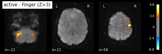
Plot thresholded z scores map.

We display it on top of the average functional image of the series (could be the anatomical image of the subject). We use arbitrarily a threshold of 3.0 in z-scale. We’ll see later how to use corrected thresholds. we show to display 3 axial views: display_mode=’z’, cut_coords=3

plot_stat_map(z_map, bg_img=mean_img, threshold=3.0,
              display_mode='z', cut_coords=3, black_bg=True,
              title='active - Finger (Z>3)')
plt.show()

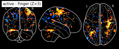
../_images/statistical_analyses_MRI_41_0.png

plot_glass_brain(z_map, threshold=3.0, black_bg=True, plot_abs=False,
                 title='active - Finger (Z>3)')
plt.show()

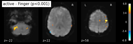
../_images/statistical_analyses_MRI_42_0.png

Statistical signifiance testing. One should worry about the statistical validity of the procedure: here we used an arbitrary threshold of 3.0 but the threshold should provide some guarantees on the risk of false detections (aka type-1 errors in statistics). One first suggestion is to control the false positive rate (fpr) at a certain level, e.g. 0.001: this means that there is.1% chance of declaring active an inactive voxel.

from nilearn.glm.thresholding import threshold_stats_img
_, threshold = threshold_stats_img(z_map, alpha=.001, height_control='fpr')
print('Uncorrected p<0.001 threshold: %.3f' % threshold)
plot_stat_map(z_map, bg_img=mean_img, threshold=threshold,
              display_mode='z', cut_coords=3, black_bg=True,
              title='active - Finger (p<0.001)')
plt.show()

Uncorrected p<0.001 threshold: 3.291

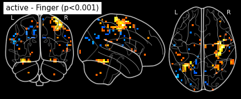
../_images/statistical_analyses_MRI_44_1.png

plot_glass_brain(z_map, threshold=threshold, black_bg=True, plot_abs=False,
                 title='active - Finger (p<0.001)')
plt.show()

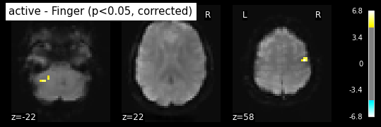
../_images/statistical_analyses_MRI_45_0.png

The problem is that with this you expect 0.001 * n_voxels to show up while they’re not active — tens to hundreds of voxels. A more conservative solution is to control the family wise errro rate, i.e. the probability of making ony one false detection, say at 5%. For that we use the so-called Bonferroni correction:

_, threshold = threshold_stats_img(z_map, alpha=.05, height_control='bonferroni')
print('Bonferroni-corrected, p<0.05 threshold: %.3f' % threshold)
plot_stat_map(z_map, bg_img=mean_img, threshold=threshold,
              display_mode='z', cut_coords=3, black_bg=True,
              title='active - Finger (p<0.05, corrected)')
plt.show()

Bonferroni-corrected, p<0.05 threshold: 4.763

../_images/statistical_analyses_MRI_47_1.png

plot_glass_brain(z_map, threshold=threshold, black_bg=True, plot_abs=False,
                 title='active - Finger (p<0.05, corrected)')
plt.show()

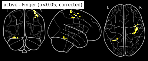
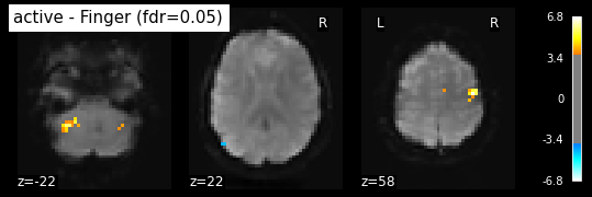
../_images/statistical_analyses_MRI_48_0.png

This is quite conservative indeed ! A popular alternative is to control the false discovery rate, i.e. the expected proportion of false discoveries among detections. This is called the false disovery rate.

_, threshold = threshold_stats_img(z_map, alpha=.05, height_control='fdr')
print('False Discovery rate = 0.05 threshold: %.3f' % threshold)
plot_stat_map(z_map, bg_img=mean_img, threshold=threshold,
              display_mode='z', cut_coords=3, black_bg=True,
              title='active - Finger (fdr=0.05)')
plt.show()

False Discovery rate = 0.05 threshold: 3.779

../_images/statistical_analyses_MRI_50_1.png

plot_glass_brain(z_map, threshold=threshold, black_bg=True, plot_abs=False,
                 title='active - Finger (fdr=0.05)')
plt.show()

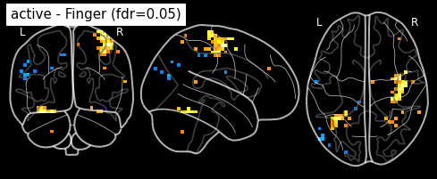
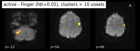
../_images/statistical_analyses_MRI_51_0.png

Finally people like to discard isolated voxels (aka “small clusters”) from these images. It is possible to generate a thresholded map with small clusters removed by providing a cluster_threshold argument. here clusters smaller than 10 voxels will be discarded.

clean_map, threshold = threshold_stats_img(
    z_map, alpha=.05, height_control='fdr', cluster_threshold=10)
plot_stat_map(clean_map, bg_img=mean_img, threshold=threshold,
              display_mode='z', cut_coords=3, black_bg=True, colorbar=False,
              title='active - Finger (fdr=0.05), clusters > 10 voxels')
plt.show()

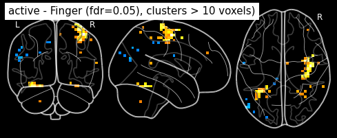
../_images/statistical_analyses_MRI_53_0.png

plot_glass_brain(z_map, threshold=threshold, black_bg=True, plot_abs=False,
                 title='active - Finger (fdr=0.05), clusters > 10 voxels)')
plt.show()

../_images/statistical_analyses_MRI_54_0.png

We can save the effect and zscore maps to the disk

z_map.to_filename(join(outdir, 'sub-01_ses-test_task-footfingerlips_space-MNI152nlin2009casym_desc-finger_zmap.nii.gz'))
eff_map.to_filename(join(outdir, 'sub-01_ses-test_task-footfingerlips_space-MNI152nlin2009casym_desc-finger_effmap.nii.gz'))

Report the found positions in a table

from nilearn.reporting import get_clusters_table
table = get_clusters_table(z_map, stat_threshold=threshold,
                           cluster_threshold=20)
print(table)

  Cluster ID     X     Y     Z  Peak Stat Cluster Size (mm3)
0          1  44.0 -12.0  58.0   6.814199               1600
1         1a  40.0 -16.0  50.0   5.930616                   

This table can be saved for future use:

table.to_csv(join(outdir, 'table.csv'))

Or use atlasreader to get even more information and informative figures:

from atlasreader import create_output
from os.path import join
create_output(join(outdir, 'sub-01_ses-test_task-footfingerlips_space-MNI152nlin2009casym_desc-finger_zmap.nii.gz'),
              cluster_extent=5, voxel_thresh=threshold)

The Python package you are importing, AtlasReader, is licensed under the
BSD-3 license; however, the atlases it uses are separately licensed under more
restrictive frameworks.
By using AtlasReader, you agree to abide by the license terms of the
individual atlases. Information on these terms can be found online at:
https://github.com/miykael/atlasreader/tree/master/atlasreader/data

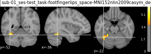
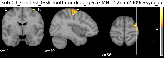
Let’s have a look at the csv file containing relevant information about the peak of each cluster. This table contains the cluster association and location of each peak, its signal value at this location, the cluster extent (in mm, not in number of voxels), as well as the membership of each peak, given a particular atlas.

peak_info = pd.read_csv('results/sub-01_ses-test_task-footfingerlips_space-MNI152nlin2009casym_desc-finger_zmap_peaks.csv')
peak_info

	cluster_id	peak_x	peak_y	peak_z	peak_value	volume_mm	aal	desikan_killiany	harvard_oxford
0	1	44	-12	58	6.81420	1600	Precentral_R	ctx-rh-precentral	63.0% Right_Precentral_Gyrus; 13.0% Right_Post...
1	2	-36	-52	-22	5.81081	960	Fusiform_L	Unknown	64.0% Left_Temporal_Occipital_Fusiform_Cortex;...
2	3	40	-4	66	6.20802	384	no_label	Unknown	16.0% Right_Precentral_Gyrus

And the clusters:

cluster_info = pd.read_csv('results/sub-01_ses-test_task-footfingerlips_space-MNI152nlin2009casym_desc-finger_zmap_clusters.csv')
cluster_info

	cluster_id	peak_x	peak_y	peak_z	cluster_mean	volume_mm	aal	desikan_killiany	harvard_oxford
0	1	44	-12	58	4.63419	1600	92.00% Precentral_R; 8.00% Postcentral_R	44.00% Unknown; 28.00% Right-Cerebral-White-Ma...	88.00% Right_Precentral_Gyrus; 12.00% Right_Po...
1	2	-36	-52	-22	4.55116	960	66.67% Fusiform_L; 20.00% Cerebelum_6_L; 13.33...	53.33% Unknown; 33.33% Left-Cerebellum-Cortex;...	86.67% Left_Temporal_Occipital_Fusiform_Cortex...
2	3	40	-4	66	4.94016	384	66.67% Frontal_Sup_2_R; 33.33% no_label	83.33% Unknown; 16.67% ctx-rh-precentral	66.67% Right_Precentral_Gyrus; 33.33% Right_Mi...

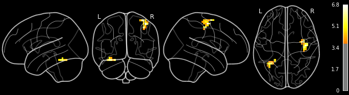
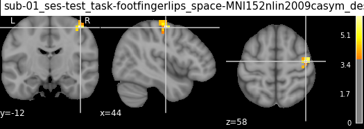
For each cluster, we also get a corresponding visualization, saved as .png:

from IPython.display import Image
Image("results/sub-01_ses-test_task-footfingerlips_space-MNI152nlin2009casym_desc-finger_zmap.png")

../_images/statistical_analyses_MRI_68_0.png

Image("results/sub-01_ses-test_task-footfingerlips_space-MNI152nlin2009casym_desc-finger_zmap_cluster01.png")

../_images/statistical_analyses_MRI_69_0.png

Image("results/sub-01_ses-test_task-footfingerlips_space-MNI152nlin2009casym_desc-finger_zmap_cluster02.png")

../_images/statistical_analyses_MRI_70_0.png

Image("results/sub-01_ses-test_task-footfingerlips_space-MNI152nlin2009casym_desc-finger_zmap_cluster03.png")

../_images/statistical_analyses_MRI_71_0.png

But wait, there’s more! There’s even a functionality to create entire GLM reports including information regarding the model and its parameters, design matrix, contrasts, etc. . All we need is the make_glm_report function from nilearn.reporting and apply it to our fitted GLM, specifying a contrast of interest.

from nilearn.reporting import make_glm_report

report = make_glm_report(fmri_glm,
                         contrasts='Finger',
                         bg_img=mean_img
                         )

Once generated, we have several options to view the GLM report: directly in the notebook, in the browser or save it as an html file:

report
#report.open_in_browser()
#report.save_as_html("GLM_report.html")

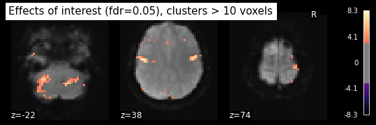
Performing an F-test¶

“active vs rest” is a typical t test: condition versus baseline. Another popular type of test is an F test in which one seeks whether a certain combination of conditions (possibly two-, three- or higher-dimensional) explains a significant proportion of the signal. Here one might for instance test which voxels are well explained by combination of the active and rest condition.

import numpy as np
effects_of_interest = np.vstack((conditions['active - Finger'], conditions['active - Lips']))
plot_contrast_matrix(effects_of_interest, design_matrix)
plt.show()

../_images/statistical_analyses_MRI_77_0.png

Specify the contrast and compute the correspoding map. Actually, the contrast specification is done exactly the same way as for t contrasts.

z_map = fmri_glm.compute_contrast(effects_of_interest,
                                  output_type='z_score')

Note that the statistic has been converted to a z-variable, which makes it easier to represent it.

clean_map, threshold = threshold_stats_img(
    z_map, alpha=.05, height_control='fdr', cluster_threshold=0)
plot_stat_map(clean_map, bg_img=mean_img, threshold=threshold,
              display_mode='z', cut_coords=3, black_bg=True,
              title='Effects of interest (fdr=0.05), clusters > 10 voxels', cmap='magma')
plt.show()

../_images/statistical_analyses_MRI_81_0.png

Evaluating models¶

While not commonly done, it’s a very good and important idea to actually evaluate your model in terms of its fit. We can do that comprehensively, yet easily through nilearn functionality. In more detail, we’re going to inspect the residuals and evaluate the predicted time series. Let’s do this for the peak voxels. At first, we have to extract them using get_clusters_table:

table = get_clusters_table(z_map, stat_threshold=1,
                           cluster_threshold=20).set_index('Cluster ID', drop=True)
table.head()

	X	Y	Z	Peak Stat	Cluster Size (mm3)
Cluster ID
1	-52.0	-12.0	38.0	8.256954	320064
1a	56.0	-8.0	34.0	7.590617
1b	40.0	-4.0	66.0	7.410259
1c	-32.0	-52.0	-22.0	6.705043
2	-12.0	-92.0	34.0	5.798149	8064

From this dataframe, we get the largest clusters and prepare a masker to extract their time series:

from nilearn import input_data

# get the largest clusters' max x, y, and z coordinates
coords = table.loc[range(1, 5), ['X', 'Y', 'Z']].values


# extract time series from each coordinate
masker = input_data.NiftiSpheresMasker(coords)

Get and check model residuals¶

We can simply obtain the residuals of the peak voxels from our fitted model via applying the prepared masker (and thus peak voxel) to the residuals our:

resid = masker.fit_transform(fmri_glm.residuals[0])

/opt/miniconda-latest/envs/neuro/lib/python3.7/site-packages/nilearn/glm/regression.py:341: FutureWarning: 'resid' from RegressionResults has been deprecated and will be removed. Please use 'residuals' instead.
  FutureWarning,

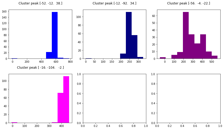
And now, we can plot them and evaluate our peak voxels based on their distribution of residuals:

# colors for each of the clusters
colors = ['blue', 'navy', 'purple', 'magenta', 'olive', 'teal']


fig2, axs2 = plt.subplots(2, 3)
axs2 = axs2.flatten()
for i in range(0, 4):
    axs2[i].set_title('Cluster peak {}\n'.format(coords[i]))
    axs2[i].hist(resid[:, i], color=colors[i])
    print('Mean residuals: {}'.format(resid[:, i].mean()))

fig2.set_size_inches(12, 7)
fig2.tight_layout()

Mean residuals: 569.9211479152854
Mean residuals: 253.89929545755146
Mean residuals: 293.17010826050404
Mean residuals: 418.41548583493346

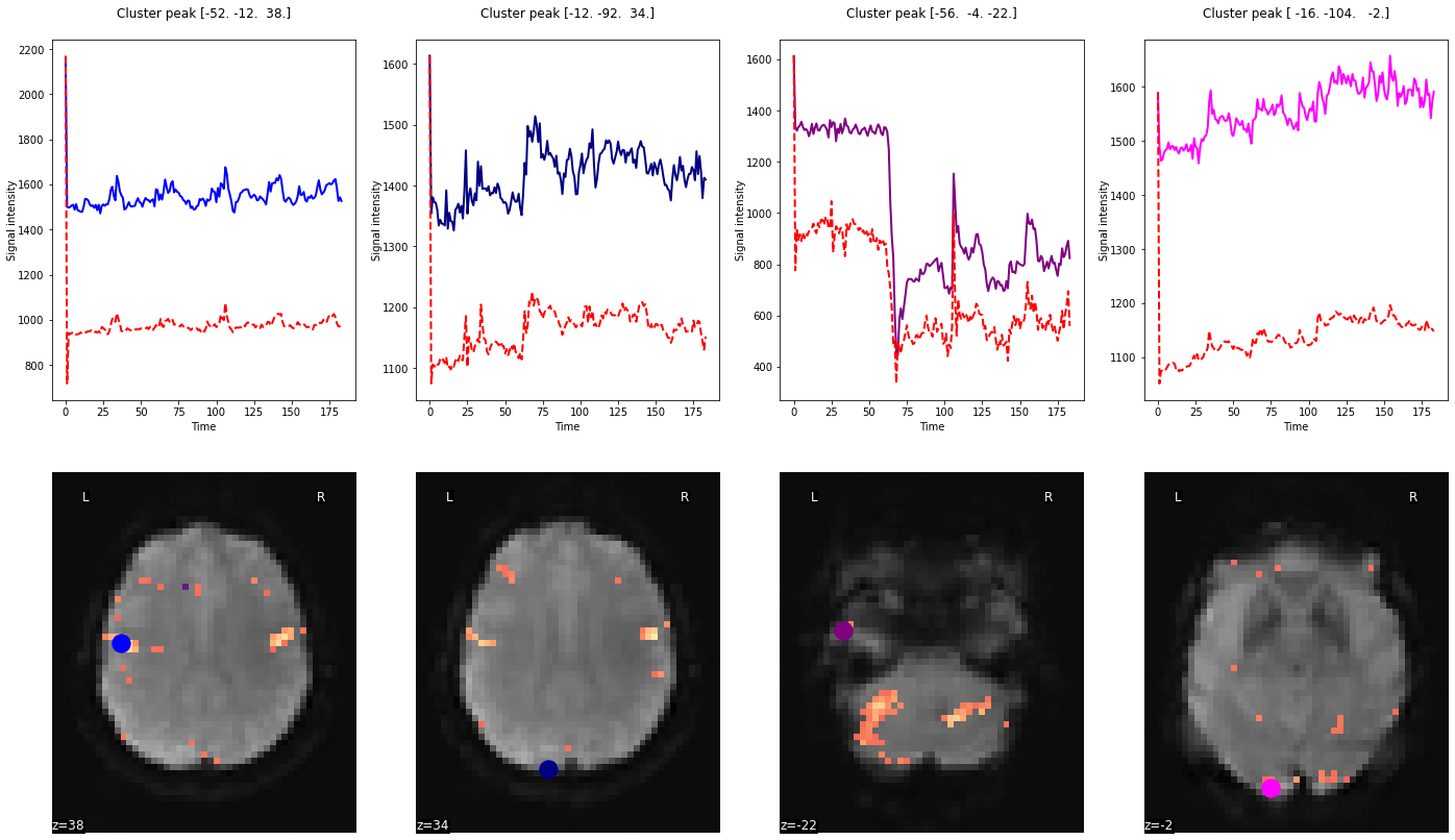
../_images/statistical_analyses_MRI_89_1.png

Get and check predicted time series¶

In order to evaluate the predicted time series we need to extract them, as well as the actual time series. To do so, we can use the masker again:

real_timeseries = masker.fit_transform(fmri_img)
predicted_timeseries = masker.fit_transform(fmri_glm.predicted[0])

Having obtained both time series, we can plot them against each other. To make it more informative, we will also visualize the respective peak voxels on the mean functional image:

from nilearn import plotting

# plot the time series and corresponding locations
fig1, axs1 = plt.subplots(2, 4)
for i in range(0, 4):
    # plotting time series
    axs1[0, i].set_title('Cluster peak {}\n'.format(coords[i]))
    axs1[0, i].plot(real_timeseries[:, i], c=colors[i], lw=2)
    axs1[0, i].plot(predicted_timeseries[:, i], c='r', ls='--', lw=2)
    axs1[0, i].set_xlabel('Time')
    axs1[0, i].set_ylabel('Signal intensity', labelpad=0)
    # plotting image below the time series
    roi_img = plotting.plot_stat_map(
        z_map, cut_coords=[coords[i][2]], threshold=3.1, figure=fig1,
        axes=axs1[1, i], display_mode='z', colorbar=False, bg_img=mean_img, cmap='magma')
    roi_img.add_markers([coords[i]], colors[i], 300)
fig1.set_size_inches(24, 14)

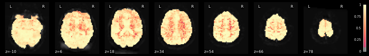
../_images/statistical_analyses_MRI_94_0.png

Plot the R-squared¶

Another option to evaluate our model is to plot the R-squared, that is the amount of variance explained through our GLM in total. While this plot will be informative, its interpretation will be limited as we can’t tell if a voxel exhibits a large R-squared because of a response to a condition in our experiment or to noise. For these things, one should employ F-Tests as shown above. However, as expected we see that the R-squared decreases the further away voxels are from the receive coils (e.g. deeper in the brain).

plotting.plot_stat_map(fmri_glm.r_square[0], bg_img=mean_img, threshold=.1,
                       display_mode='z', cut_coords=7, cmap='magma')

<nilearn.plotting.displays.ZSlicer at 0x7fba685b8610>

../_images/statistical_analyses_MRI_96_1.png

Group level statistics¶

Now that we’ve explored the individual level analysis quite a bit, one might ask: but what about group level statistics? No problem at all, nilearn’s GLM functionality of course supports this as well. As in other software packages, we need to repeat the individual level analysis for each subject to obtain the same contrast images, that we can submit to a group level analysis.

Run individual level analysis for multiple participants¶

By now, we know how to do this easily. Let’s use a simple for loop to repeat the analysis from above for sub-02 and sub-03.

for subject in ['02', '03']:

    # set the fMRI image
    fmri_img = '/data/ds000114/derivatives/fmriprep/sub-%s/ses-test/func/sub-%s_ses-test_task-fingerfootlips_space-MNI152nlin2009casym_desc-preproc_bold.nii.gz' %(subject, subject)
    
    # read in the events 
    events = pd.read_table('/data/ds000114/task-fingerfootlips_events.tsv')
    
    # read in the confounds
    confounds = pd.read_table('/data/ds000114/derivatives/fmriprep/sub-%s/ses-test/func/sub-%s_ses-test_task-fingerfootlips_bold_desc-confounds_timeseries.tsv' %(subject, subject))
    
    # restrict the to be included confounds to a subset
    confounds_glm = confounds[['WhiteMatter', 'GlobalSignal', 'FramewiseDisplacement', 'X', 'Y', 'Z', 'RotX', 'RotY', 'RotZ']].replace(np.nan, 0)
    
    # run the GLM
    fmri_glm = fmri_glm.fit(fmri_img, events, confounds_glm)
    
    # compute the contrast as a z-map
    z_map = fmri_glm.compute_contrast(conditions['active - Finger'],
                                  output_type='z_score')
    
    # save the z-map
    z_map.to_filename(join(outdir, 'sub-%s_ses-test_task-footfingerlips_space-MNI152nlin2009casym_desc-finger_zmap.nii.gz' %subject))

/opt/miniconda-latest/envs/neuro/lib/python3.7/site-packages/nilearn/_utils/glm.py:276: UserWarning: Matrix is singular at working precision, regularizing...
  warn('Matrix is singular at working precision, regularizing...')

Define a group level model¶

As we now have the same contrast from multiple subjects we can define our group level model. At first, we need to gather the individual contrast maps:

from glob import glob
list_z_maps = glob(join(outdir, 'sub-*_ses-test_task-footfingerlips_space-MNI152nlin2009casym_desc-finger_zmap.nii.gz'))


list_z_maps

['results/sub-01_ses-test_task-footfingerlips_space-MNI152nlin2009casym_desc-finger_zmap.nii.gz',
 'results/sub-02_ses-test_task-footfingerlips_space-MNI152nlin2009casym_desc-finger_zmap.nii.gz',
 'results/sub-03_ses-test_task-footfingerlips_space-MNI152nlin2009casym_desc-finger_zmap.nii.gz']

Great! The next step includes the definition of a design matrix. As we want to run a simple one-sample t-test, we just need to indicate as many 1 as we have z-maps:

design_matrix = pd.DataFrame([1] * len(list_z_maps),
                             columns=['intercept'])

Believe it or not, that’s all it takes. Within the next step we can already set and run our model. It’s basically identical to the First_level_model: we need to define the images and design matrix:

from nilearn.glm.second_level import SecondLevelModel
second_level_model = SecondLevelModel()
second_level_model = second_level_model.fit(list_z_maps,
                                            design_matrix=design_matrix)

The same holds true for contrast computation:

z_map_group = second_level_model.compute_contrast(output_type='z_score')

What do we get? After defining a liberal threshold of p<0.001 (uncorrected), we can plot our computed group level contrast image:

from scipy.stats import norm
p001_unc = norm.isf(0.001)

plotting.plot_glass_brain(z_map_group, colorbar=True, threshold=p001_unc,
                          title='Group Finger tapping (unc p<0.001)',
                          plot_abs=False, display_mode='x', cmap='magma')
plotting.show()

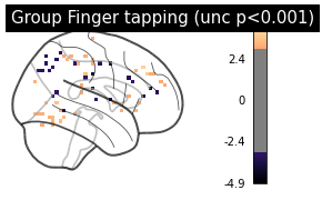
../_images/statistical_analyses_MRI_108_0.png

Well, not much going there…But please remember we also just included three participants. Besides this rather simple model, nilearn’s GLM functionality of course also allows you to run paired t-test, two-sample t-test, F-test, etc. . As shown above, you also can define different thresholds and multiple comparison corrections. There’s yet another cool thing we didn’t talk about. It’s possible to run analyses in a rather automated way if your dataset is in BIDS.

Performing statistical analyses on BIDS datasets¶

Even though model specification and running was comparably easy and straightforward, it can be even better. Nilearn’s GLM functionality actually enables you to define models for multiple participants through one function by leveraging the BIDS standard. More precisely, the function first_level_from_bids takes the same input arguments as First_Level_model (e.g. t_r, hrf_model, high_pass, etc.), but through defining the BIDS raw and derivatives folder, as well as a task and space label automatically extracts all information necessary to run individual level models and creates the model itself for all participants.

from nilearn.glm.first_level import first_level_from_bids

data_dir = '/data/ds000114/'
task_label = 'fingerfootlips'
space_label = 'MNI152nlin2009casym'
derivatives_folder = 'derivatives/fmriprep'

models, models_run_imgs, models_events, models_confounds = \
    first_level_from_bids(data_dir, task_label, space_label,
                          smoothing_fwhm=5.0,
                          derivatives_folder=derivatives_folder, 
                          t_r=2.5, 
                          noise_model='ar1',
                          hrf_model='spm',
                          drift_model='cosine',
                          high_pass=1./160,
                          signal_scaling=False,
                          minimize_memory=False)

/opt/miniconda-latest/envs/neuro/lib/python3.7/site-packages/nilearn/glm/first_level/first_level.py:811: UserWarning: RepetitionTime given in model_init as 2
  warn('RepetitionTime given in model_init as %d' % t_r)
/opt/miniconda-latest/envs/neuro/lib/python3.7/site-packages/nilearn/glm/first_level/first_level.py:813: UserWarning: slice_time_ref is 0 percent of the repetition time
  'time' % slice_time_ref)

Done, let’s check if things work as expected. As an example, we will have a look at the information for sub-01. We’re going to start with the images.

import os
print([os.path.basename(run) for run in models_run_imgs[0]])

['sub-01_ses-test_task-fingerfootlips_space-MNI152nlin2009casym_desc-preproc_bold.nii.gz']

Looks good. How about confounds?

print(models_confounds[0][0])

     WhiteMatter  GlobalSignal   stdDVARS  non-stdDVARS  vx-wisestdDVARS  \
    59.958244    296.705627        NaN           NaN              NaN   
    -0.992987     -6.791035  10.967166    359.572876        15.125442   
     0.121577     -8.960917   0.965478     31.654449         1.251122   
    -3.207463    -15.836485   0.568300     18.632469         0.933274   
    -3.531865    -16.072039   0.412484     13.523833         1.089049   
..           ...           ...        ...           ...              ...   
  -1.131588      6.617327   0.796877     26.126665         0.812802   
  -2.441096      3.395323   0.606146     19.873285         0.689635   
  -4.028681     -0.000021   0.725305     23.780071         0.768956   
  -4.716608      0.375874   0.549176     18.005463         0.654098   
  -2.884027      2.981873   0.582871     19.110176         0.675460   

     FramewiseDisplacement  tCompCor00  tCompCor01  tCompCor02  tCompCor03  \
                    NaN   -0.945194    0.178691   -0.008839    0.023860   
               0.522051    0.095183   -0.081205    0.043344   -0.067988   
               0.053361    0.039534   -0.048124    0.023519   -0.009606   
               0.079333    0.064448   -0.049706    0.013449   -0.031648   
               0.030417    0.058324   -0.050976    0.013930   -0.027509   
..                     ...         ...         ...         ...         ...   
             0.162573    0.001240   -0.007174   -0.044028   -0.010630   
             0.080021    0.003447    0.006033   -0.038060    0.003348   
             0.195117    0.008511    0.018631   -0.045767    0.042005   
             0.085730    0.009503    0.000066   -0.031858   -0.026816   
             0.453545    0.004254   -0.009564   -0.043303   -0.052722   

     ...  aCompCor02  aCompCor03  aCompCor04  aCompCor05             X  \
  ...    0.001226   -0.070598    0.040292   -0.004502 -6.811590e-03   
  ...   -0.006754    0.102960   -0.020727    0.005408 -1.198610e-09   
  ...   -0.006754    0.096988   -0.022278   -0.102161  0.000000e+00   
  ...   -0.036826    0.078502    0.003200   -0.112108  0.000000e+00   
  ...   -0.024400    0.069612    0.006408   -0.060869  2.562640e-10   
..   ...         ...         ...         ...         ...           ...   
...   -0.076143    0.074762    0.004733    0.020203 -5.966000e-01   
...    0.006482    0.081220    0.004589   -0.054566 -6.161150e-01   
...    0.019911   -0.027145   -0.028081    0.013844 -6.761900e-01   
...    0.026724    0.012923    0.025031    0.012589 -6.877110e-01   
...   -0.014826    0.072763    0.044807   -0.027618 -5.796220e-01   

            Y         Z      RotX      RotY      RotZ  
  0.000000  0.000000  0.000000 -0.000000  0.000000  
 -0.035396  0.386632  0.001864 -0.000000  0.000000  
 -0.019626  0.383440  0.001176 -0.000000  0.000000  
 -0.032375  0.430492  0.001567 -0.000000  0.000000  
 -0.032767  0.404579  0.001485 -0.000000  0.000000  
..        ...       ...       ...       ...       ...  
0.258395  1.762940  0.000232  0.003428 -0.013078  
0.237964  1.772880  0.000388  0.003602 -0.013351  
0.216604  1.814620 -0.000184  0.003883 -0.013937  
0.198889  1.825820 -0.000529  0.004307 -0.013800  
0.244931  1.756250  0.000987  0.003099 -0.011926  

[184 rows x 24 columns]

Ah, the NaN again. Let’s fix those as we did last time, but for all participants.

models_confounds_no_nan = []

for confounds in models_confounds:
    models_confounds_no_nan.append(confounds[0].fillna(0)[['WhiteMatter', 'GlobalSignal', 'FramewiseDisplacement', 'X', 'Y', 'Z', 'RotX', 'RotY', 'RotZ']])

Last but not least: how do the events look?

print(models_events[0][0]['trial_type'].value_counts())

Lips      5
Foot      5
Finger    5
Name: trial_type, dtype: int64

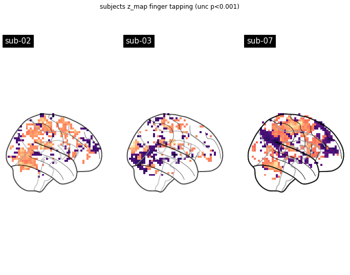
Fantastic, now we’re ready to run our models. With a little zip magic this is done without a problem. We also going to compute z-maps as before and plot them side by side.

from nilearn import plotting
import matplotlib.pyplot as plt

models_fitted = [] 

fig, axes = plt.subplots(nrows=1, ncols=3, figsize=(12, 8.5))
model_and_args = zip(models, models_run_imgs, models_events, models_confounds_no_nan)
for midx, (model, imgs, events, confounds) in enumerate(model_and_args):
    # fit the GLM
    model.fit(imgs, events, confounds)
        
    models_fitted.append(model)
    
    # compute the contrast of interest
    zmap = model.compute_contrast('Finger')
    plotting.plot_glass_brain(zmap, colorbar=False, threshold=p001_unc,
                              title=('sub-' + model.subject_label),
                              axes=axes[int(midx-1)],
                              plot_abs=False, display_mode='x', cmap='magma')
fig.suptitle('subjects z_map finger tapping (unc p<0.001)')
plotting.show()

/opt/miniconda-latest/envs/neuro/lib/python3.7/site-packages/nilearn/_utils/glm.py:276: UserWarning: Matrix is singular at working precision, regularizing...
  warn('Matrix is singular at working precision, regularizing...')
/opt/miniconda-latest/envs/neuro/lib/python3.7/site-packages/nilearn/plotting/displays.py:1110: MatplotlibDeprecationWarning: Adding an axes using the same arguments as a previous axes currently reuses the earlier instance.  In a future version, a new instance will always be created and returned.  Meanwhile, this warning can be suppressed, and the future behavior ensured, by passing a unique label to each axes instance.
  .3 * (x1 - x0), y1 - y0], aspect='equal')

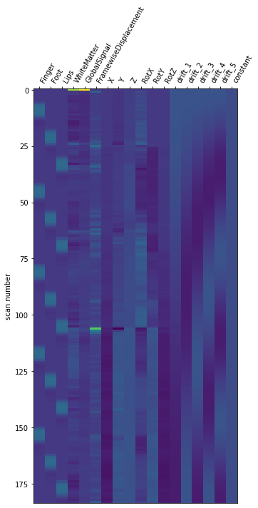
../_images/statistical_analyses_MRI_121_1.png

That looks about right. However, let’s also check the design matrix

from nilearn.plotting import plot_design_matrix
plot_design_matrix(models_fitted[0].design_matrices_[0])

<AxesSubplot:label='conditions', ylabel='scan number'>

../_images/statistical_analyses_MRI_123_1.png

and contrast matrix.

plot_contrast_matrix('Finger', models_fitted[0].design_matrices_[0])
plt.show()

../_images/statistical_analyses_MRI_125_0.png

Nothing to complain here and thus we can move on to the group level model. Instead of assembling contrast images from each participant, we also have the option to simply provide the fitted individual level models as input.

from nilearn.glm.second_level import SecondLevelModel
second_level_input = models_fitted

That’s all it takes and we can run our group level model again.

second_level_model = SecondLevelModel()
second_level_model = second_level_model.fit(second_level_input)

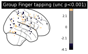
And after computing the contrast

zmap = second_level_model.compute_contrast(
    first_level_contrast='Finger')

we can plot the results again.

plotting.plot_glass_brain(zmap, colorbar=True, threshold=p001_unc,
                          title='Group Finger tapping (unc p<0.001)',
                          plot_abs=False, display_mode='x', cmap='magma')
plotting.show()

../_images/statistical_analyses_MRI_133_0.png

If we want, we can also easily inspect results via an interactive surface plot as shown a few times before (please note that we change the thresholds as we have very little voxels remaining due to the limited number of participants):

from nilearn.plotting import view_img_on_surf
view_img_on_surf(zmap, threshold='75%', cmap='magma')

That’s all for now. Please note, that we only showed a small part of what’s possible. Make sure to check the documentation and the examples it includes. We hope we could show you how powerful nilearn will be through including GLM functionality. While there’s already a lot you can do, there will be even more in the future.

Introduction to pybids

Functional connectivity and resting state

MRI analysis in Python using Nipype, Nilearn and more