Introduction to Statistics in python¶

In this section, we will cover how you can use Python to do some statistics. There are many packages to do so, but we will focus on four:

This notebook is strongly based on the scipy-lectures.org section about statistics.

Data representation and interaction¶

Data as a table¶

The setting that we consider for statistical analysis is that of multiple observations or samples described by a set of different attributes or features. The data can than be seen as a 2D table, or matrix, with columns giving the different attributes of the data, and rows the observations. For example purposes, we will make use of phenotypic information within a dataset from OpenNeuro, provided as part of the following publication:

Keren H., Zheng C., Jangraw D.C., Chang K., Vitale A., Rutledge R.B., Pereira F., Nielson D.M., Stringaris A. (2021). The temporal representation of experience in subjective mood. eLife, 2021;10:e62051.

It contains sex, age, handedness, group id, Mood and Feelings Questionnaire total scores and Snaith-Hamilton Pleasure Scale total scores for a fair amount of participants.

We will use curl to gather the respective file:

%%bash
curl https://openneuro.org/crn/datasets/ds003709/snapshots/1.0.0/files/participants.tsv -o /data/participants_stats.tsv

  % Total    % Received % Xferd  Average Speed   Time    Time     Time  Current
                                 Dload  Upload   Total   Spent    Left  Speed

  0     0    0     0    0     0      0      0 --:--:-- --:--:-- --:--:--     0
  0     0    0     0    0     0      0      0 --:--:-- --:--:-- --:--:--     0
100  1761    0  1761    0     0  14238      0 --:--:-- --:--:-- --:--:-- 14201

!head /data/participants_stats.tsv

participant_id	sex	age	handedness	group	MFQ	SHAPS
sub-20900	M	17	RIGHT	HV	0.0	1.0
sub-22686	M	16	RIGHT	HV	2.0	10.0
sub-23017	F	17	RIGHT	MDD	15.0	6.0
sub-23108	F	16	RIGHT	HV	0.0	7.0
sub-23303	F	16	RIGHT	HV	0.0	0.0
sub-23399	F	17	RIGHT	MDD	1.0	14.0
sub-23520	F	17	RIGHT	MDD	7.0	22.0
sub-23540	F	16	RIGHT	MDD	5.0	21.0
sub-23546	F	17	RIGHT	MDD	1.0	0.0

The pandas data-frame¶

Creating dataframes: reading data files or converting arrays¶

Reading from a CSV file¶

Using the above CSV file that gives observations of brain size and weight and IQ (Willerman et al. 1991), the data are a mixture of numerical and categorical values::

import pandas as pd
data = pd.read_csv('/data/participants_stats.tsv', sep='\t', na_values=".")
data

	participant_id	sex	age	handedness	group	MFQ	SHAPS
0	sub-20900	M	17	RIGHT	HV	0.0	1.0
1	sub-22686	M	16	RIGHT	HV	2.0	10.0
2	sub-23017	F	17	RIGHT	MDD	15.0	6.0
3	sub-23108	F	16	RIGHT	HV	0.0	7.0
4	sub-23303	F	16	RIGHT	HV	0.0	0.0
5	sub-23399	F	17	RIGHT	MDD	1.0	14.0
6	sub-23520	F	17	RIGHT	MDD	7.0	22.0
7	sub-23540	F	16	RIGHT	MDD	5.0	21.0
8	sub-23546	F	17	RIGHT	MDD	1.0	0.0
9	sub-23549	M	16	RIGHT	MDD	4.0	20.0
10	sub-23564	F	16	RIGHT	MDD	2.0	15.0
11	sub-23576	F	15	RIGHT	MDD	9.0	4.0
12	sub-23593	F	15	RIGHT	MDD	16.0	18.0
13	sub-23607	F	17	RIGHT	MDD	6.0	2.0
14	sub-23613	F	14	RIGHT	HV	NaN	NaN
15	sub-23625	F	14	RIGHT	MDD	8.0	8.0
16	sub-23639	F	17	RIGHT	HV	4.0	1.0
17	sub-23643	F	17	RIGHT	MDD	13.0	17.0
18	sub-23649	F	15	RIGHT	MDD	15.0	16.0
19	sub-23652	M	16	RIGHT	MDD	8.0	17.0
20	sub-23673	F	17	RIGHT	HV	0.0	5.0
21	sub-23674	F	15	RIGHT	MDD	6.0	9.0
22	sub-23689	F	18	RIGHT	MDD	5.0	3.0
23	sub-23717	M	16	AMBIDEXTROUS	MDD	9.0	14.0
24	sub-23718	F	17	RIGHT	MDD	NaN	NaN
25	sub-23720	F	16	RIGHT	MDD	5.0	12.0
26	sub-23757	F	14	RIGHT	MDD	1.0	1.0
27	sub-23780	F	18	RIGHT	MDD	15.0	3.0
28	sub-23783	F	14	LEFT	MDD	NaN	NaN
29	sub-23798	F	15	RIGHT	MDD	8.0	8.0
30	sub-23814	F	13	RIGHT	MDD	20.0	10.0
31	sub-23817	F	15	LEFT	HV	0.0	0.0
32	sub-23820	F	16	RIGHT	HV	0.0	0.0
33	sub-23823	M	17	RIGHT	MDD	5.0	21.0
34	sub-23830	M	16	LEFT	MDD	14.0	26.0
35	sub-23834	F	13	RIGHT	HV	2.0	2.0
36	sub-23843	F	16	RIGHT	HV	1.0	5.0
37	sub-23856	F	12	RIGHT	HV	1.0	14.0
38	sub-23866	M	16	RIGHT	HV	4.0	15.0
39	sub-23867	F	14	AMBIDEXTROUS	MDD	11.0	25.0
40	sub-23880	F	17	RIGHT	HV	0.0	0.0
41	sub-23890	F	14	RIGHT	HV	0.0	2.0
42	sub-23901	M	15	RIGHT	HV	NaN	0.0
43	sub-23903	F	15	RIGHT	MDD	16.0	11.0
44	sub-23905	F	16	RIGHT	HV	4.0	10.0
45	sub-23919	M	14	LEFT	MDD	0.0	1.0
46	sub-23937	F	15	AMBIDEXTROUS	HV	0.0	0.0
47	sub-23943	F	16	RIGHT	HV	8.0	NaN
48	sub-23951	F	13	RIGHT	MDD	8.0	11.0
49	sub-23952	M	15	RIGHT	MDD	5.0	16.0
50	sub-23969	F	15	RIGHT	HV	NaN	NaN

Creating from arrays¶

A pandas.DataFrame can also be seen as a dictionary of 1D ‘series’, eg arrays or lists. If we have 3 numpy arrays:

import numpy as np
t = np.linspace(-6, 6, 20)
sin_t = np.sin(t)
cos_t = np.cos(t)

We can expose them as a pandas.DataFrame:

pd.DataFrame({'t': t, 'sin': sin_t, 'cos': cos_t}).head()

	t	sin	cos
0	-6.000000	0.279415	0.960170
1	-5.368421	0.792419	0.609977
2	-4.736842	0.999701	0.024451
3	-4.105263	0.821291	-0.570509
4	-3.473684	0.326021	-0.945363

Other inputs: pandas can input data from SQL, excel files, or other formats. See the pandas documentation.

Manipulating data¶

data is a pandas.DataFrame, that resembles R’s dataframe:

data.shape    # 51 rows and 7 columns

(51, 7)

data.columns  # It has columns

Index(['participant_id', 'sex', 'age', 'handedness', 'group', 'MFQ', 'SHAPS'], dtype='object')

print(data['group'].head())  # Columns can be addressed by name

   HV
   HV
  MDD
   HV
   HV
Name: group, dtype: object

# Simpler selector
data[data['group'] == 'HV']['MFQ'].mean()

1.5294117647058822

Note: For a quick view on a large dataframe, use its describe pandas.DataFrame.describe.

data.describe()

	age	MFQ	SHAPS
count	51.000000	46.000000	46.000000
mean	15.568627	5.739130	9.195652
std	1.360219	5.511341	7.759208
min	12.000000	0.000000	0.000000
25%	15.000000	1.000000	2.000000
50%	16.000000	5.000000	8.500000
75%	17.000000	8.000000	15.000000
max	18.000000	20.000000	26.000000

# Frequency count for a given column
data['age'].value_counts()

  15
  12
  11
   7
   3
   2
   1
Name: age, dtype: int64

# Dummy-code # of group (i.e., get N-binary columns)
pd.get_dummies(data['group'])[:15]

	HV	MDD
0	1	0
1	1	0
2	0	1
3	1	0
4	1	0
5	0	1
6	0	1
7	0	1
8	0	1
9	0	1
10	0	1
11	0	1
12	0	1
13	0	1
14	1	0

The split-apply-combine pattern¶

A very common data processing strategy is to…
- Split the dataset into groups
- Apply some operation(s) to each group
- (Optionally) combine back into one dataset

Pandas provides powerful and fast tools for this. For example the groupby function.

groupby: splitting a dataframe on values of categorical variables:

groupby_group = data.groupby('group')
for group, value in groupby_group['MFQ']:
     print((group, value.mean()))

('HV', 1.5294117647058822)
('MDD', 8.206896551724139)

groupby_group is a powerful object that exposes many operations on the resulting group of dataframes:

groupby_group.mean()

	age	MFQ	SHAPS
group
HV	15.450000	1.529412	4.235294
MDD	15.645161	8.206897	12.103448

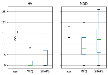
Plotting data¶

Pandas comes with some plotting tools (pandas.tools.plotting, using matplotlib behind the scene) to display statistics of the data in dataframes.

For example, let’s use boxplot (in this case even groupby_group.boxplot) to better understand the structure of the data.

%matplotlib inline
groupby_group.boxplot(column=['age', 'MFQ', 'SHAPS']);

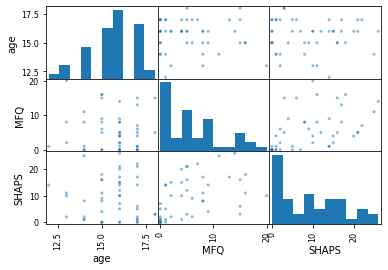
Scatter matrices¶

pd.plotting.scatter_matrix(data[['age', 'MFQ', 'SHAPS']]);

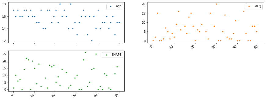
Plot content of a dataset¶

data.head()

	participant_id	sex	age	handedness	group	MFQ	SHAPS
0	sub-20900	M	17	RIGHT	HV	0.0	1.0
1	sub-22686	M	16	RIGHT	HV	2.0	10.0
2	sub-23017	F	17	RIGHT	MDD	15.0	6.0
3	sub-23108	F	16	RIGHT	HV	0.0	7.0
4	sub-23303	F	16	RIGHT	HV	0.0	0.0

data.plot(lw=0, marker='.', subplots=True, layout=(-1, 2), figsize=(15, 6));

Pingouin is an open-source statistical package written in Python 3 and based mostly on Pandas and NumPy.¶

ANOVAs: one- and two-ways, repeated measures, mixed, ancova
Post-hocs tests and pairwise comparisons
Robust correlations
Partial correlation, repeated measures correlation and intraclass correlation
Linear/logistic regression and mediation analysis
Bayesian T-test and Pearson correlation
Tests for sphericity, normality and homoscedasticity
Effect sizes and power analysis
Parametric/bootstrapped confidence intervals around an effect size or a correlation coefficient
Circular statistics
Plotting: Bland-Altman plot, Q-Q plot, etc…

Pingouin is designed for users who want simple yet exhaustive statistical functions.

**material scavenged from 10 minutes to Pingouin and the pingouin docs ¶

import pingouin as pg

Measures of correlation

“In the broadest sense correlation is any statistical association, though in common usage it most often refers to how close two variables are to having a linear relationship with each other” - Wikipedia

When talking about correlation, we commonly mean the Pearson correlation coefficient, also referred to as Pearson’s r

pearson_correlation = pg.corr(data['MFQ'], data['SHAPS'])
display(pearson_correlation)
cor_coeeficient = pearson_correlation['r']
n =  len(data) # sample size

	n	r	CI95%	r2	adj_r2	p-val	BF10	power
pearson	45	0.457	[0.19, 0.66]	0.209	0.171	0.001601	16.321	0.898

Test summary¶

‘n’ : Sample size (after NaN removal)
‘outliers’ : number of outliers (only for ‘shepherd’ or ‘skipped’)
‘r’ : Correlation coefficient
‘CI95’ : 95% parametric confidence intervals
‘r2’ : R-squared
‘adj_r2’ : Adjusted R-squared
‘p-val’ : one or two tailed p-value
‘BF10’ : Bayes Factor of the alternative hypothesis (Pearson only)
‘power’ : achieved power of the test (= 1 - type II error)

Before we calculate: `Testing statistical premises`¶

Statistical procedures can be classfied into either parametric or non parametric prcedures, which require different necessary preconditions to be met in order to show consistent/robust results. Generally people assume that their data follows a gaussian distribution, which allows for parametric tests to be run. Nevertheless it is essential to first test the distribution of your data to decide if the assumption of normally distributed data holds, if this is not the case we would have to switch to non parametric tests.

Shapiro Wilk normality test ¶

Standard procedure to test for normal distribution. Tests if the distribution of you data deviates significtanly from a normal distribution. returns:

normal : boolean True if x comes from a normal distribution.
p : float P-value.

# Return a boolean (true if normal) and the associated p-value
pg.normality(data['MFQ'])

(True, 1.0)

Henze-Zirkler multivariate normality test ¶

Same procedure for multivariate normal distributions

returns

normal : boolean True if X comes from a multivariate normal distribution.
p : float P-value.

# Return a boolean (true if normal) and the associated p-value
import numpy as np
np.random.seed(123)
mean, cov, n = [4, 6], [[1, .5], [.5, 1]], 30
X = np.random.multivariate_normal(mean, cov, n)
pg.multivariate_normality(X, alpha=.05)

(True, 0.7523511059223016)

Mauchly test for sphericity ¶

“Sphericity is the condition where the variances of the differences between all combinations of related groups (levels) are equal. Violation of sphericity is when the variances of the differences between all combinations of related groups are not equal.” - https://statistics.laerd.com/statistical-guides/sphericity-statistical-guide.php

returns

spher : boolean True if data have the sphericity property.
W : float Test statistic
chi_sq : float Chi-square statistic
ddof : int Degrees of freedom
p : float P-value.

pg.sphericity(data)

(False, 0.002, 302.823, 20, 2.142051582323624e-52)

Testing for homoscedasticity ¶

“In statistics, a sequence or a vector of random variables is homoscedastic /ˌhoʊmoʊskəˈdæstɪk/ if all random variables in the sequence or vector have the same finite variance.” - wikipedia

returns:

equal_var : boolean True if data have equal variance.
p : float P-value.

Note: This function first tests if the data are normally distributed using the Shapiro-Wilk test. If yes, then the homogeneity of variances is measured using the Bartlett test. If the data are not normally distributed, the Levene test, which is less sensitive to departure from normality, is used.

np.random.seed(123)
# Scale = standard deviation of the distribution.
array_1 = np.random.normal(loc=0, scale=1., size=100)
array_2 = np.random.normal(loc=0, scale=0.8,size=100)
print(np.var(array_1), np.var(array_2))

pg.homoscedasticity(array_1, array_2, alpha=.05)

1.2729265592243306 0.6022425373276372

(False, 0.0)

Parametric tests¶

Student’s t-test: the simplest statistical test¶

1-sample t-test: testing the value of a population mean¶

tests if the population mean of data is likely to be equal to a given value (technically if observations are drawn from a Gaussian distributions of given population mean).

pingouin.ttest returns the T_statistic, the p-value, the [degrees of freedom](https://en.wikipedia.org/wiki/Degrees_of_freedom_(statistics), the Cohen d effect size, the achieved [power](https://en.wikipedia.org/wiki/Power_(statistics)) of the test ( = 1 - type II error (beta) = P(Reject H0|H1 is true)), and the Bayes Factor of the alternative hypothesis

pg.ttest(data['MFQ'],0)

	T	p-val	dof	tail	cohen-d	power	BF10
T-test	7.063	8.228161e-09	45	two-sided	1.041	1.0	1527145.713

2-sample t-test: testing for difference across populations¶

We have seen above that the mean MFQ in the MDD and HV populations were different. To test if this is significant, we do a 2-sample t-test:

MDD_MFQ = data[data['group'] == 'MDD']['MFQ']
HV_MFQ = data[data['group'] == 'HV']['MFQ']

pg.ttest(MDD_MFQ, HV_MFQ)

	T	p-val	dof	dof-corr	tail	cohen-d	power	BF10
T-test	5.866	6.718419e-07	44	40.991061	two-sided	1.486	0.997	22256.489

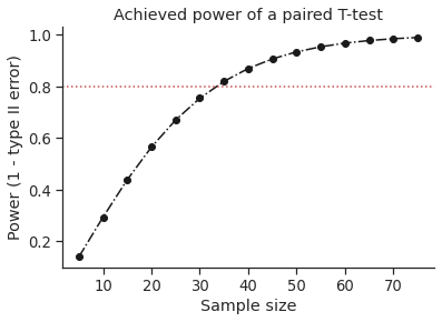
Plot achieved power of a paired T-test¶

Plot the curve of achieved power given the effect size (Cohen d) and the sample size of a paired T-test.

import matplotlib.pyplot as plt
import seaborn as sns
sns.set(style='ticks', context='notebook', font_scale=1.2)

d = 0.5  # Fixed effect size
n = np.arange(5, 80, 5)  # Incrementing sample size

# Compute the achieved power
pwr = pg.power_ttest(d=d, n=n, contrast='paired', tail='two-sided')

# Start the plot
plt.plot(n, pwr, 'ko-.')
plt.axhline(0.8, color='r', ls=':')
plt.xlabel('Sample size')
plt.ylabel('Power (1 - type II error)')
plt.title('Achieved power of a paired T-test')
sns.despine()

Non parametric tests:¶

Unlike the parametric test these do not require the assumption of normal distributions.

“Mann-Whitney U Test (= Wilcoxon rank-sum test). It is the non-parametric version of the independent T-test. Mwu tests the hypothesis that data in x and y are samples from continuous distributions with equal medians. The test assumes that x and y are independent. This test corrects for ties and by default uses a continuity correction.” - mwu-function

Test summary

‘W-val’ : W-value
‘p-val’ : p-value
‘RBC’ : matched pairs rank-biserial correlation (effect size)
‘CLES’ : common language effect size

pg.mwu(MDD_MFQ, HV_MFQ)

	U-val	p-val	RBC	CLES
MWU	442.0	0.000008	-0.793103	0.872211

“Wilcoxon signed-rank test is the non-parametric version of the paired T-test.

The Wilcoxon signed-rank test tests the null hypothesis that two related paired samples come from the same distribution. A continuity correction is applied by default.” - wilcoxon - func

# example from the function definition
# Wilcoxon test on two related samples.
x = [20, 22, 19, 20, 22, 18, 24, 20]
y = [38, 37, 33, 29, 14, 12, 20, 22]
print("Medians = %.2f - %.2f" % (np.median(x), np.median(y)))
pg.wilcoxon(x, y, tail='two-sided')

Medians = 20.00 - 25.50

/opt/miniconda-latest/envs/neuro/lib/python3.7/site-packages/scipy/stats/morestats.py:2879: UserWarning: Sample size too small for normal approximation.
  warnings.warn("Sample size too small for normal approximation.")

	W-val	p-val	RBC	CLES
Wilcoxon	9.0	0.043089	0.5	0.609375

`scipy.stats` - Hypothesis testing: comparing two groups¶

For simple statistical tests, it is also possible to use the scipy.stats sub-module of scipy.

from scipy import stats

1-sample t-test: testing the value of a population mean¶

scipy.stats.ttest_1samp tests if the population mean of data is likely to be equal to a given value (technically if observations are drawn from a Gaussian distributions of given population mean). It returns the T statistic, and the p-value (see the function’s help):

stats.ttest_1samp(data['MFQ'].dropna(), 0)

Ttest_1sampResult(statistic=7.062650755155121, pvalue=8.228161269771835e-09)

With a p-value of 8^-09 we can claim that the population mean for the MFQ is not 0.

2-sample t-test: testing for difference across populations¶

We have seen above that the mean MFQ in the MDD and HV populations were different. To test if this is significant, we do a 2-sample t-test with scipy.stats.ttest_ind:

stats.ttest_ind(MDD_MFQ.dropna(), HV_MFQ.dropna())

Ttest_indResult(statistic=4.863337342528167, pvalue=1.5121907363581306e-05)

Paired tests: repeated measurements on the same indivuals¶

MFQ and SHAPS are measures of interest. Let us test if they are significantly different. We can use a 2 sample test:

stats.ttest_ind(data['MFQ'].dropna(), data['SHAPS'].dropna())

Ttest_indResult(statistic=-2.4632108396344363, pvalue=0.01567217083007739)

The problem with this approach is that it forgets that there are links between observations: MFQ and SHAPS are measured on the same individuals.

Thus the variance due to inter-subject variability is confounding, and can be removed, using a “paired test”, or “repeated measures test”:

stats.ttest_rel(data['MFQ'].dropna(), data['SHAPS'].dropna())

Ttest_relResult(statistic=-3.006858621511653, pvalue=0.004308118483154467)

This is equivalent to a 1-sample test on the difference::

stats.ttest_1samp(data['MFQ'].dropna() - data['SHAPS'].dropna(), 0)

Ttest_1sampResult(statistic=nan, pvalue=nan)

T-tests assume Gaussian errors. We can use a Wilcoxon signed-rank test, that relaxes this assumption:

stats.wilcoxon(data['MFQ'].dropna(), data['SHAPS'].dropna())

WilcoxonResult(statistic=177.0, pvalue=0.004985029827378135)

Note: The corresponding test in the non paired case is the Mann–Whitney U test, scipy.stats.mannwhitneyu.

`statsmodels` - use “formulas” to specify statistical models in Python¶

Use statsmodels to perform linear models, multiple factors or analysis of variance.

A simple linear regression¶

Given two set of observations, x and y, we want to test the hypothesis that y is a linear function of x.

In other terms:

\(y = x * coef + intercept + e\)

where \(e\) is observation noise. We will use the statsmodels module to:

Fit a linear model. We will use the simplest strategy, ordinary least squares (OLS).
Test that \(coef\) is non zero.

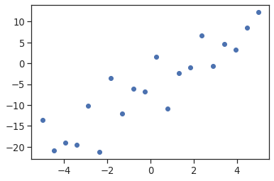
First, we generate simulated data according to the model:

import numpy as np
import matplotlib.pyplot as plt

x = np.linspace(-5, 5, 20)
np.random.seed(1)

# normal distributed noise
y = -5 + 3*x + 4 * np.random.normal(size=x.shape)

# Create a data frame containing all the relevant variables
data = pd.DataFrame({'x': x, 'y': y})

plt.plot(x, y, 'o');

Then we specify an OLS model and fit it:

from statsmodels.formula.api import ols
model = ols("y ~ x", data).fit()

Note: For more about “formulas” for statistics in Python, see the statsmodels documentation.

We can inspect the various statistics derived from the fit::

print(model.summary())

                            OLS Regression Results                            
==============================================================================
Dep. Variable:                      y   R-squared:                       0.804
Model:                            OLS   Adj. R-squared:                  0.794
Method:                 Least Squares   F-statistic:                     74.03
Date:                Sun, 17 Oct 2021   Prob (F-statistic):           8.56e-08
Time:                        16:14:47   Log-Likelihood:                -57.988
No. Observations:                  20   AIC:                             120.0
Df Residuals:                      18   BIC:                             122.0
Df Model:                           1                                         
Covariance Type:            nonrobust                                         
==============================================================================
                 coef    std err          t      P>|t|      [0.025      0.975]
------------------------------------------------------------------------------
Intercept     -5.5335      1.036     -5.342      0.000      -7.710      -3.357
x              2.9369      0.341      8.604      0.000       2.220       3.654
==============================================================================
Omnibus:                        0.100   Durbin-Watson:                   2.956
Prob(Omnibus):                  0.951   Jarque-Bera (JB):                0.322
Skew:                          -0.058   Prob(JB):                        0.851
Kurtosis:                       2.390   Cond. No.                         3.03
==============================================================================

Notes:
[1] Standard Errors assume that the covariance matrix of the errors is correctly specified.

Terminology¶

Statsmodels uses a statistical terminology: the y variable in statsmodels is called endogenous while the x variable is called exogenous. This is discussed in more detail here. To simplify, y (endogenous) is the value you are trying to predict, while x (exogenous) represents the features you are using to make the prediction.

Categorical variables: comparing groups or multiple categories¶

Let us go back to our data. We can write a comparison between MFQ of MDD and HV groups using a linear model:

data = pd.read_csv('/data/participants_stats.tsv', sep='\t', na_values=".")

model = ols("MFQ ~ group + 1", data).fit()
print(model.summary())

                            OLS Regression Results                            
==============================================================================
Dep. Variable:                    MFQ   R-squared:                       0.350
Model:                            OLS   Adj. R-squared:                  0.335
Method:                 Least Squares   F-statistic:                     23.65
Date:                Sun, 17 Oct 2021   Prob (F-statistic):           1.51e-05
Time:                        16:14:54   Log-Likelihood:                -133.38
No. Observations:                  46   AIC:                             270.8
Df Residuals:                      44   BIC:                             274.4
Df Model:                           1                                         
Covariance Type:            nonrobust                                         
================================================================================
                   coef    std err          t      P>|t|      [0.025      0.975]
--------------------------------------------------------------------------------
Intercept        1.5294      1.090      1.403      0.168      -0.668       3.727
group[T.MDD]     6.6775      1.373      4.863      0.000       3.910       9.445
==============================================================================
Omnibus:                        2.463   Durbin-Watson:                   1.836
Prob(Omnibus):                  0.292   Jarque-Bera (JB):                1.930
Skew:                           0.502   Prob(JB):                        0.381
Kurtosis:                       3.012   Cond. No.                         3.05
==============================================================================

Notes:
[1] Standard Errors assume that the covariance matrix of the errors is correctly specified.

Tips on specifying model¶

Forcing categorical - the ‘group’ variable is automatically detected as a categorical variable, and thus each of its different values is treated as different entities.

An integer column can be forced to be treated as categorical using:

model = ols('MFQ ~ C(group)', data).fit()

Intercept: We can remove the intercept using - 1 in the formula, or force the use of an intercept using + 1.

Link to t-tests between different MFQ and SHAPS¶

To compare different types of our measurements of interest, we need to create a "long-form" table, listing them, where their type is indicated by a categorical variable:

data_mfq = pd.DataFrame({'MOI': data['MFQ'], 'type': 'MFQ'})
data_shaps = pd.DataFrame({'MOI': data['SHAPS'], 'type': 'SHAPS'})
data_long = pd.concat((data_mfq, data_shaps))
print(data_long[::8])

     MOI   type
  0.0    MFQ
  1.0    MFQ
 4.0    MFQ
 NaN    MFQ
 0.0    MFQ
 0.0    MFQ
 8.0    MFQ
 14.0  SHAPS
 2.0  SHAPS
 9.0  SHAPS
 8.0  SHAPS
14.0  SHAPS
 1.0  SHAPS

model = ols("MOI ~ type", data_long).fit()
print(model.summary())

                            OLS Regression Results                            
==============================================================================
Dep. Variable:                    MOI   R-squared:                       0.063
Model:                            OLS   Adj. R-squared:                  0.053
Method:                 Least Squares   F-statistic:                     6.067
Date:                Sun, 17 Oct 2021   Prob (F-statistic):             0.0157
Time:                        16:14:56   Log-Likelihood:                -304.93
No. Observations:                  92   AIC:                             613.9
Df Residuals:                      90   BIC:                             618.9
Df Model:                           1                                         
Covariance Type:            nonrobust                                         
=================================================================================
                    coef    std err          t      P>|t|      [0.025      0.975]
---------------------------------------------------------------------------------
Intercept         5.7391      0.992      5.784      0.000       3.768       7.710
type[T.SHAPS]     3.4565      1.403      2.463      0.016       0.669       6.244
==============================================================================
Omnibus:                        6.740   Durbin-Watson:                   1.892
Prob(Omnibus):                  0.034   Jarque-Bera (JB):                6.017
Skew:                           0.548   Prob(JB):                       0.0494
Kurtosis:                       2.391   Cond. No.                         2.62
==============================================================================

Notes:
[1] Standard Errors assume that the covariance matrix of the errors is correctly specified.

We can see that we retrieve the same values for t-test and corresponding p-values for the effect of the type of MOI than the previous t-test:

stats.ttest_ind(data['MFQ'].dropna(), data['SHAPS'].dropna())

Ttest_indResult(statistic=-2.4632108396344363, pvalue=0.01567217083007739)

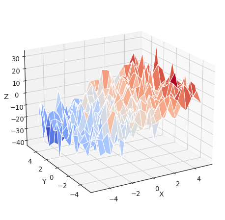
Multiple Regression: including multiple factors¶

Consider a linear model explaining a variable z (the dependent variable) with 2 variables x and y:

\(z = x \, c_1 + y \, c_2 + i + e\)

Such a model can be seen in 3D as fitting a plane to a cloud of (x, y, z) points (see the following figure).

from mpl_toolkits.mplot3d import Axes3D
x = np.linspace(-5, 5, 21)

# We generate a 2D grid
X, Y = np.meshgrid(x, x)

# To get reproducable values, provide a seed value
np.random.seed(1)

# Z is the elevation of this 2D grid
Z = -5 + 3*X - 0.5*Y + 8 * np.random.normal(size=X.shape)

# Plot the data
fig = plt.figure(figsize=(8, 8))
ax = fig.gca(projection='3d')
surf = ax.plot_surface(X, Y, Z, cmap=plt.cm.coolwarm,
                       rstride=1, cstride=1)
ax.view_init(20, -120)
ax.set_xlabel('X')
ax.set_ylabel('Y')
ax.set_zlabel('Z')

Text(0.5, 0, 'Z')

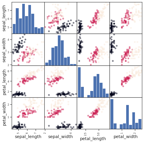
Example: the iris dataset¶

Sepal and petal size tend to be related: bigger flowers are bigger! But is there, in addition, a systematic effect of species?

from pandas.plotting import scatter_matrix

#Load the data
data = sns.load_dataset('iris')

# Express the names as categories
categories = pd.Categorical(data['species'])

# The parameter 'c' is passed to plt.scatter and will control the color
scatter_matrix(data, c=categories.codes, marker='o', figsize=(8, 8))

# Plot figure
fig.suptitle("blue: setosa, green: versicolor, red: virginica", size=13)
plt.show()

model = ols('sepal_width ~ species + petal_length', data).fit()
print(model.summary())

                            OLS Regression Results                            
==============================================================================
Dep. Variable:            sepal_width   R-squared:                       0.486
Model:                            OLS   Adj. R-squared:                  0.476
Method:                 Least Squares   F-statistic:                     46.08
Date:                Sun, 17 Oct 2021   Prob (F-statistic):           5.14e-21
Time:                        16:14:59   Log-Likelihood:                -37.808
No. Observations:                 150   AIC:                             83.62
Df Residuals:                     146   BIC:                             95.66
Df Model:                           3                                         
Covariance Type:            nonrobust                                         
=========================================================================================
                            coef    std err          t      P>|t|      [0.025      0.975]
-----------------------------------------------------------------------------------------
Intercept                 2.9919      0.099     30.206      0.000       2.796       3.188
species[T.versicolor]    -1.4927      0.181     -8.264      0.000      -1.850      -1.136
species[T.virginica]     -1.6741      0.255     -6.557      0.000      -2.179      -1.170
petal_length              0.2983      0.060      4.932      0.000       0.179       0.418
==============================================================================
Omnibus:                        3.167   Durbin-Watson:                   1.771
Prob(Omnibus):                  0.205   Jarque-Bera (JB):                3.214
Skew:                          -0.121   Prob(JB):                        0.200
Kurtosis:                       3.675   Cond. No.                         54.0
==============================================================================

Notes:
[1] Standard Errors assume that the covariance matrix of the errors is correctly specified.

Post-hoc hypothesis testing: analysis of variance (ANOVA)¶

In the above iris example, we wish to test if the petal length is different between versicolor and virginica, after removing the effect of sepal width. This can be formulated as testing the difference between the coefficient associated to versicolor and virginica in the linear model estimated above (it is an Analysis of Variance, ANOVA. For this, we write a vector of ‘contrast’ on the parameters estimated: we want to test "name[T.versicolor] - name[T.virginica]", with an F-test:

print(model.f_test([0, 1, -1, 0]))

<F test: F=array([[3.26191465]]), p=0.07296614041660528, df_denom=146, df_num=1>

Is this difference significant?

`seaborn` - use visualization for statistical exploration¶

Seaborn combines simple statistical fits with plotting on pandas dataframes.

Let us consider a data giving wages and many other personal information on 500 individuals (Berndt, ER. The Practice of Econometrics. 1991. NY:Addison-Wesley) which we will gather using a small function based on the scipy tutorials.

def download_wages_data():
    
    import urllib
    import os
    
    import pandas as pd

    if not os.path.exists('wages.txt'):
        # Download the file if it is not present
        urllib.request.urlretrieve('http://lib.stat.cmu.edu/datasets/CPS_85_Wages',
                           'wages.txt')

    # Give names to the columns
    names = [
        'EDUCATION: Number of years of education',
        'SOUTH: 1=Person lives in South, 0=Person lives elsewhere',
        'SEX: 1=Female, 0=Male',
        'EXPERIENCE: Number of years of work experience',
        'UNION: 1=Union member, 0=Not union member',
        'WAGE: Wage (dollars per hour)',
        'AGE: years',
        'RACE: 1=Other, 2=Hispanic, 3=White',
        'OCCUPATION: 1=Management, 2=Sales, 3=Clerical, 4=Service, 5=Professional, 6=Other',
        'SECTOR: 0=Other, 1=Manufacturing, 2=Construction',
        'MARR: 0=Unmarried,  1=Married',
    ]

    short_names = [n.split(':')[0] for n in names]

    data = pd.read_csv('wages.txt', skiprows=27, skipfooter=6, sep=None,
                           header=None)
    data.columns = short_names

    # Log-transform the wages, because they typically are increased with
    # multiplicative factors
    import numpy as np
    data['WAGE'] = np.log10(data['WAGE'])
    
    return data

import pandas as pd
data = download_wages_data()
data.head()

/opt/miniconda-latest/envs/neuro/lib/python3.7/site-packages/ipykernel_launcher.py:31: ParserWarning: Falling back to the 'python' engine because the 'c' engine does not support skipfooter; you can avoid this warning by specifying engine='python'.

	EDUCATION	SEX	EXPERIENCE	WAGE	AGE	RACE	OCCUPATION	SECTOR	MARR
0	8	1	21	0.707570	35	2	6	1	1
1	9	1	42	0.694605	57	3	6	1	1
2	12	0	1	0.824126	19	3	6	1	0
3	12	0	4	0.602060	22	3	6	0	0
4	12	0	17	0.875061	35	3	6	0	1

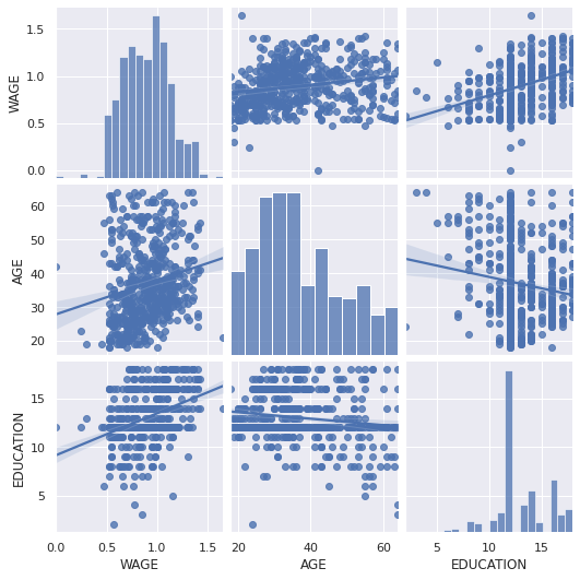
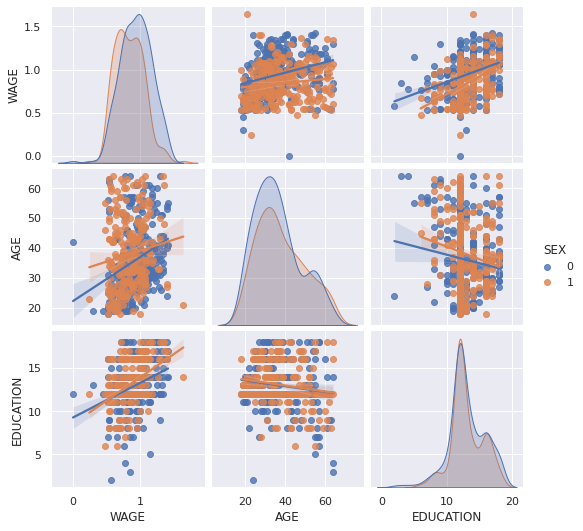
Pairplot: scatter matrices¶

We can easily have an intuition on the interactions between continuous variables using seaborn.pairplot to display a scatter matrix:

import seaborn
seaborn.set()
seaborn.pairplot(data, vars=['WAGE', 'AGE', 'EDUCATION'], kind='reg')

<seaborn.axisgrid.PairGrid at 0x7fe5c444a350>

Categorical variables can be plotted as the hue:

seaborn.pairplot(data, vars=['WAGE', 'AGE', 'EDUCATION'], kind='reg', hue='SEX')

<seaborn.axisgrid.PairGrid at 0x7fe5c2183e10>

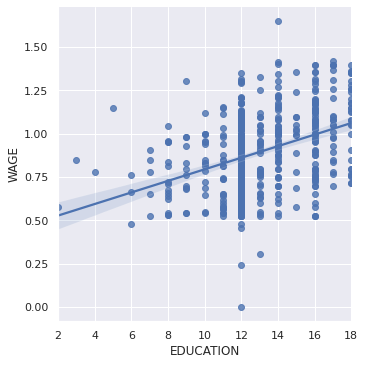
lmplot: plotting a univariate regression¶

A regression capturing the relation between one variable and another, e.g. wage and eduction, can be plotted using seaborn.lmplot:

seaborn.lmplot(y='WAGE', x='EDUCATION', data=data)

<seaborn.axisgrid.FacetGrid at 0x7fe5c23700d0>

Robust regression¶

Given that, in the above plot, there seems to be a couple of data points that are outside of the main cloud to the right, they might be outliers, not representative of the population, but driving the regression.

To compute a regression that is less sensitive to outliers, one must use a robust model. This is done in seaborn using robust=True in the plotting functions, or in statsmodels by replacing the use of the OLS by a “Robust Linear Model”, statsmodels.formula.api.rlm.

Testing for interactions¶

Do wages increase more with education for people with dark hair than with light hair?

seaborn.lmplot(y='WAGE', x='EDUCATION', hue='SEX', data=data)

<seaborn.axisgrid.FacetGrid at 0x7fe5caa1f9d0>

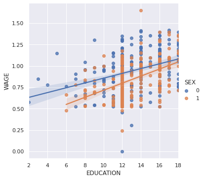
The plot above is made of two different fits. We need to formulate a single model that tests for a variance of slope across the population. This is done via an “interaction”.

from statsmodels.formula.api import ols
result = ols(formula='WAGE ~ EDUCATION + SEX + EDUCATION * SEX', data=data).fit()
print(result.summary())

                            OLS Regression Results                            
==============================================================================
Dep. Variable:                   WAGE   R-squared:                       0.198
Model:                            OLS   Adj. R-squared:                  0.194
Method:                 Least Squares   F-statistic:                     43.72
Date:                Sun, 17 Oct 2021   Prob (F-statistic):           2.94e-25
Time:                        16:15:09   Log-Likelihood:                 88.503
No. Observations:                 534   AIC:                            -169.0
Df Residuals:                     530   BIC:                            -151.9
Df Model:                           3                                         
Covariance Type:            nonrobust                                         
=================================================================================
                    coef    std err          t      P>|t|      [0.025      0.975]
---------------------------------------------------------------------------------
Intercept         0.5748      0.058      9.861      0.000       0.460       0.689
EDUCATION         0.0281      0.004      6.411      0.000       0.019       0.037
SEX              -0.2750      0.093     -2.972      0.003      -0.457      -0.093
EDUCATION:SEX     0.0134      0.007      1.919      0.056      -0.000       0.027
==============================================================================
Omnibus:                        4.838   Durbin-Watson:                   1.825
Prob(Omnibus):                  0.089   Jarque-Bera (JB):                5.000
Skew:                          -0.156   Prob(JB):                       0.0821
Kurtosis:                       3.356   Cond. No.                         170.
==============================================================================

Notes:
[1] Standard Errors assume that the covariance matrix of the errors is correctly specified.

Can we conclude that education benefits people with dark hair more than people with light hair?

Take home messages¶

Hypothesis testing and p-value give you the significance of an effect / difference
Formulas (with categorical variables) enable you to express rich links in your data
Visualizing your data and simple model fits matters!
Conditioning (adding factors that can explain all or part of the variation) is an important modeling aspect that changes the interpretation.

Introduction to Visualization in python

Introduction to scikit-learn & scikit-image

MRI analysis in Python using Nipype, Nilearn and more

Introduction to Statistics in python¶

Data representation and interaction¶

Data as a table¶

The pandas data-frame¶

Creating dataframes: reading data files or converting arrays¶

Reading from a CSV file¶

Creating from arrays¶

Manipulating data¶

The split-apply-combine pattern¶

Plotting data¶

Scatter matrices¶

Plot content of a dataset¶

Pingouin is an open-source statistical package written in Python 3 and based mostly on Pandas and NumPy.¶

**material scavenged from 10 minutes to Pingouin and the pingouin docs¶

Test summary¶

Before we calculate: Testing statistical premises¶

Shapiro Wilk normality test¶

Henze-Zirkler multivariate normality test¶

Mauchly test for sphericity¶

Testing for homoscedasticity¶

Parametric tests¶

Student’s t-test: the simplest statistical test¶

1-sample t-test: testing the value of a population mean¶

2-sample t-test: testing for difference across populations¶

Plot achieved power of a paired T-test¶

Non parametric tests:¶

scipy.stats - Hypothesis testing: comparing two groups¶

1-sample t-test: testing the value of a population mean¶

2-sample t-test: testing for difference across populations¶

Paired tests: repeated measurements on the same indivuals¶

statsmodels - use “formulas” to specify statistical models in Python¶

A simple linear regression¶

Terminology¶

Categorical variables: comparing groups or multiple categories¶

Tips on specifying model¶

Link to t-tests between different MFQ and SHAPS¶

Multiple Regression: including multiple factors¶

Example: the iris dataset¶

Post-hoc hypothesis testing: analysis of variance (ANOVA)¶

seaborn - use visualization for statistical exploration¶

Pairplot: scatter matrices¶

lmplot: plotting a univariate regression¶

Robust regression¶

Testing for interactions¶

Take home messages¶

**material scavenged from 10 minutes to Pingouin and the pingouin docs ¶

Before we calculate: `Testing statistical premises`¶

Shapiro Wilk normality test ¶

Henze-Zirkler multivariate normality test ¶

Mauchly test for sphericity ¶

Testing for homoscedasticity ¶

`scipy.stats` - Hypothesis testing: comparing two groups¶

`statsmodels` - use “formulas” to specify statistical models in Python¶

`seaborn` - use visualization for statistical exploration¶