Introduction to NumPy
Disclaimer: Most of the content in this notebook is coming from www.scipy-lectures.org
NumPy
NumPy is the fundamental package for scientific computing with Python. It is the basic building block of most data analysis in Python and contains highly optimized routines for creating and manipulating arrays.
Everything revolves around numpy arrays
Scipyadds a bunch of useful science and engineering routines that operate on numpy arrays. E.g. signal processing, statistical distributions, image analysis, etc.pandasadds powerful methods for manipulating numpy arrays. Like data frames in R - but typically faster.scikit-learnsupports state-of-the-art machine learning over numpy arrays. Inputs and outputs of virtually all functions are numpy arrays.If you want many more short exercises than the ones in this notebook - you can find 100 of them here
NumPy arrays vs Python arrays
NumPy arrays look very similar to Pyhon arrays.
import numpy as np
a = np.array([0, 1, 2, 3])
a
array([0, 1, 2, 3])
So, why is this useful? NumPy arrays are memory-efficient containers that provide fast numerical operations. We can show this very quickly by running a simple computation on the same two arrays.
L = range(1000)

# Computing the power of the first 1000 numbers with Python arrays
%timeit [i**2 for i in L]
187 µs ± 11.8 µs per loop (mean ± std. dev. of 7 runs, 10000 loops each)
a = np.array(L)

# Computing the power of the first 1000 numbers with Numpy arrays
%timeit a**2
1.28 µs ± 38.7 ns per loop (mean ± std. dev. of 7 runs, 1000000 loops each)
Creating arrays
Manual construction of arrays
You can create NumPy arrays manually almost in the same way as in Python in general.
2-D, 3-D, …
b = np.array([[0, 1, 2], [3, 4, 5]])    # 2 x 3 array
b
array([[0, 1, 2],
       [3, 4, 5]])
b.shape
(2, 3)
c = np.array([[[1], [2]], [[3], [4]]])
c
array([[[1],
        [2]],

       [[3],
        [4]]])
c.shape
(2, 2, 1)
Functions for creating arrays
In practice, we rarely enter items one by one. Therefore, NumPy offers many different helper functions.
Evenly spaced
a = np.arange(10) # 0 .. n-1  (!)
a
array([0, 1, 2, 3, 4, 5, 6, 7, 8, 9])
b = np.arange(1, 9, 2) # start, end (exclusive), step
b
array([1, 3, 5, 7])
… or by number of points
c = np.linspace(0, 1, 6)   # start, end, num-points
c
array([0. , 0.2, 0.4, 0.6, 0.8, 1. ])
d = np.linspace(0, 1, 5, endpoint=False)
d
array([0. , 0.2, 0.4, 0.6, 0.8])
Common arrays
a = np.ones((3, 3))  # reminder: (3, 3) is a tuple
a
array([[1., 1., 1.],
       [1., 1., 1.],
       [1., 1., 1.]])
b = np.zeros((2, 2))
b
array([[0., 0.],
       [0., 0.]])
c = np.eye(3)
c
array([[1., 0., 0.],
       [0., 1., 0.],
       [0., 0., 1.]])
d = np.diag(np.array([1, 2, 3, 4]))
d
array([[1, 0, 0, 0],
       [0, 2, 0, 0],
       [0, 0, 3, 0],
       [0, 0, 0, 4]])
np.random: random numbers (Mersenne Twister PRNG)
a = np.random.rand(4)       # uniform in [0, 1]
a
array([0.72812914, 0.2888934 , 0.16006505, 0.57169499])
b = np.random.randn(4)      # Gaussian
b
array([-1.06432023, 0.56855512, -0.8431078 , 0.01674151])
np.random.seed(1234) # Setting the random seed
Basic data types
You may have noticed that, in some instances, array elements are displayed with a trailing dot (e.g. 2. vs 2). This is due to a difference in the data-type used:
a = np.array([1, 2, 3])
a.dtype
dtype('int64')
b = np.array([1., 2., 3.])
b.dtype
dtype('float64')
Different data-types allow us to store data more compactly in memory, but most of the time we simply work with floating point numbers. Note that, in the example above, NumPy auto-detects the data-type from the input.
You can explicitly specify which data-type you want:
c = np.array([1, 2, 3], dtype=float)
c.dtype
dtype('float64')
The default data type is floating point:
a = np.ones((3, 3))
a.dtype
dtype('float64')
There are also other types:
# Complex
d = np.array([1+2j, 3+4j, 5+6*1j])
d.dtype
dtype('complex128')
# Bool
e = np.array([True, False, False, True])
e.dtype
dtype('bool')
# Strings
f = np.array(['Bonjour', 'Hello', 'Hallo',])
f.dtype     # <--- strings containing max. 7 letters
dtype('<U7')
And much more…
int32int64uint32uint64
Indexing and slicing
The items of an array can be accessed and assigned to the same way as other Python sequences (e.g. lists):
a = np.arange(10)
a
array([0, 1, 2, 3, 4, 5, 6, 7, 8, 9])
a[0], a[2], a[-1]
(0, 2, 9)
Warning: Indices begin at 0, like other Python sequences (and C/C++). In contrast, in Fortran or Matlab, indices begin at 1.
The usual python idiom for reversing a sequence is supported:
a[::-1]
array([9, 8, 7, 6, 5, 4, 3, 2, 1, 0])
For multidimensional arrays, indexes are tuples of integers:
a = np.diag(np.arange(3))
a
array([[0, 0, 0],
       [0, 1, 0],
       [0, 0, 2]])
a[1, 1]
1
a[2, 1] = 10 # third line, second column
a
array([[ 0,  0,  0],
       [ 0,  1,  0],
       [ 0, 10,  2]])
a[1]
array([0, 1, 0])
Note
In 2D, the first dimension corresponds to rows, the second to columns.
For multidimensional
a,a[0]is interpreted by taking all elements in the unspecified dimensions.
Slicing: Arrays, like other Python sequences can also be sliced
a = np.arange(10)
a
array([0, 1, 2, 3, 4, 5, 6, 7, 8, 9])
a[2:9:3] # [start:end:step]
array([2, 5, 8])
Note that the last index is not included!
a[:4]
array([0, 1, 2, 3])
All three slice components are not required: by default, start is 0,
end is the last and step is 1:
a[1:3]
array([1, 2])
a[::2]
array([0, 2, 4, 6, 8])
a[3:]
array([3, 4, 5, 6, 7, 8, 9])
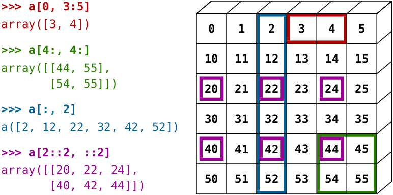
A small illustrated summary of NumPy indexing and slicing…
You can also combine assignment and slicing:
a = np.arange(10)
a[5:] = 10
a
array([ 0, 1, 2, 3, 4, 10, 10, 10, 10, 10])
b = np.arange(5)
a[5:] = b[::-1]
a
array([0, 1, 2, 3, 4, 4, 3, 2, 1, 0])
Fancy indexing
NumPy arrays can be indexed with slices, but also with boolean or integer arrays (masks). This method is called fancy indexing. It creates copies not views.
Using boolean masks
np.random.seed(3)
a = np.random.randint(0, 21, 15)
a
array([10, 3, 8, 0, 19, 10, 11, 9, 10, 6, 0, 20, 12, 7, 14])
(a % 3 == 0)
array([False,  True, False,  True, False, False, False,  True, False,
        True,  True, False,  True, False, False])
mask = (a % 3 == 0)
extract_from_a = a[mask] # or,  a[a%3==0]
extract_from_a           # extract a sub-array with the mask
array([ 3, 0, 9, 6, 0, 12])
Indexing with a mask can be very useful to assign a new value to a sub-array:
a[a % 3 == 0] = -1
a
array([10, -1, 8, -1, 19, 10, 11, -1, 10, -1, -1, 20, -1, 7, 14])
Indexing with an array of integers
a = np.arange(0, 100, 10)
a
array([ 0, 10, 20, 30, 40, 50, 60, 70, 80, 90])
Indexing can be done with an array of integers, where the same index is repeated several time:
a[[2, 3, 2, 4, 2]] # note: [2, 3, 2, 4, 2] is a Python list
array([20, 30, 20, 40, 20])
New values can be assigned with this kind of indexing:
a[[9, 7]] = -100
a
array([ 0, 10, 20, 30, 40, 50, 60, -100, 80, -100])
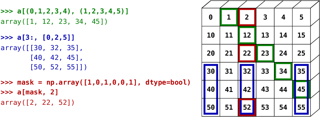
The image below illustrates various fancy indexing applications:
Elementwise operations
NumPy provides many elementwise operations that are much quicker than comparable list comprehension in plain Python.
Basic operations
With scalars:
a = np.array([1, 2, 3, 4])
a + 1
array([2, 3, 4, 5])
2**a
array([ 2, 4, 8, 16])
All arithmetic operates elementwise:
b = np.ones(4) + 1
a - b
array([-1., 0., 1., 2.])
a * b
array([2., 4., 6., 8.])
j = np.arange(5)
2**(j + 1) - j
array([ 2, 3, 6, 13, 28])
Array multiplication is not matrix multiplication
c = np.ones((3, 3))
c * c                   # NOT matrix multiplication!
array([[1., 1., 1.],
       [1., 1., 1.],
       [1., 1., 1.]])
# Matrix multiplication
c.dot(c)
array([[3., 3., 3.],
       [3., 3., 3.],
       [3., 3., 3.]])
Other operations
Comparisons
a = np.array([1, 2, 3, 4])
b = np.array([4, 2, 2, 4])
a == b
array([False, True, False, True])
a > b
array([False, False, True, False])
Array-wise comparisons:
a = np.array([1, 2, 3, 4])
b = np.array([4, 2, 2, 4])
c = np.array([1, 2, 3, 4])
np.array_equal(a, b)
False
np.array_equal(a, c)
True
Logical operations
a = np.array([1, 1, 0, 0], dtype=bool)
b = np.array([1, 0, 1, 0], dtype=bool)
np.logical_or(a, b)
array([ True, True, True, False])
np.logical_and(a, b)
array([ True, False, False, False])
Transcendental functions
a = np.arange(5)
np.sin(a)
array([ 0. , 0.84147098, 0.90929743, 0.14112001, -0.7568025 ])
np.log(a)
/opt/miniconda-latest/envs/neuro/lib/python3.7/site-packages/ipykernel_launcher.py:1: RuntimeWarning: divide by zero encountered in log
  """Entry point for launching an IPython kernel.
array([ -inf, 0. , 0.69314718, 1.09861229, 1.38629436])
np.exp(a)
array([ 1. , 2.71828183, 7.3890561 , 20.08553692, 54.59815003])
Shape mismatches
a = np.arange(4)
# NBVAL_SKIP
a + np.array([1, 2])
---------------------------------------------------------------------------
ValueError                                Traceback (most recent call last)
<ipython-input-67-d870f1bba8f8> in <module>
      1 # NBVAL_SKIP
----> 2 a + np.array([1, 2])

ValueError: operands could not be broadcast together with shapes (4,) (2,)
Broadcasting? We’ll return to that later.
Transposition
a = np.triu(np.ones((3, 3)), 1)
a
array([[0., 1., 1.],
       [0., 0., 1.],
       [0., 0., 0.]])
a.T
array([[0., 0., 0.],
       [1., 0., 0.],
       [1., 1., 0.]])
The transposition is a view
As a result, the following code is wrong and will not make a matrix symmetric:
>>> a += a.T
It will work for small arrays (because of buffering) but fail for large one, in unpredictable ways.
Basic reductions
NumPy offers many quick functions to compute things like sum, mean, max etc.
Computing sums
x = np.array([1, 2, 3, 4])
np.sum(x)
10
Note: Certain NumPy functions can be also written at the end of an Numpy array.
x.sum()
10
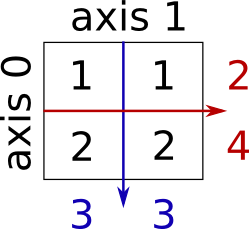
Sum by rows and by columns:
x = np.array([[1, 1], [2, 2]])
x
array([[1, 1],
       [2, 2]])
x.sum(axis=0) # columns (first dimension)
array([3, 3])
x.sum(axis=1) # rows (second dimension)
array([2, 4])
Other reductions
Like, mean, std, cumsum etc. works the same way (and take axis=).
Extrema
x = np.array([1, 3, 2])
x.min()
1
x.max()
3
x.argmin() # index of minimum
0
x.argmax() # index of maximum
1
Logical operations
np.all([True, True, False])
False
np.any([True, True, False])
True
Can be used for array comparisons:
a = np.zeros((100, 100))
np.any(a != 0)
False
np.all(a == a)
True
a = np.array([1, 2, 3, 2])
b = np.array([2, 2, 3, 2])
c = np.array([6, 4, 4, 5])
((a <= b) & (b <= c)).all()
True
Statistics
x = np.array([1, 2, 3, 1])
y = np.array([[1, 2, 3], [5, 6, 1]])
x.mean()
1.75
np.median(x)
1.5
np.median(y, axis=-1) # last axis
array([2., 5.])
x.std() # full population standard dev.
0.82915619758885
… and many more (best to learn as you go).
Broadcasting
Basic operations on
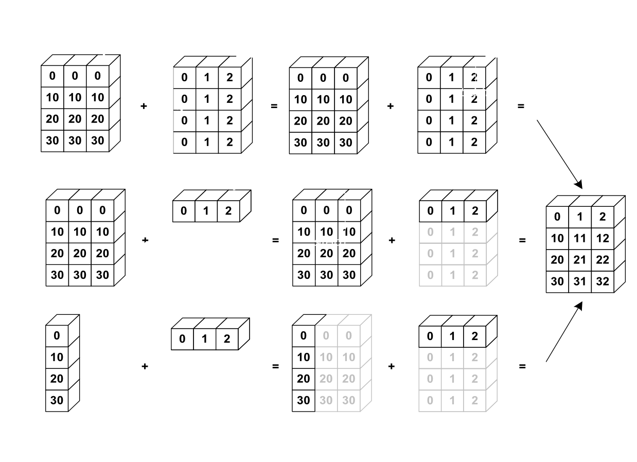
numpyarrays (addition, etc.) are elementwiseThis works on arrays of the same size. Nevertheless, It’s also possible to do operations on arrays of different sizes if NumPy can transform these arrays so that they all have the same size: this conversion is called broadcasting.
The image below gives an example of broadcasting:
Let’s verify this:
a = np.tile(np.arange(0, 40, 10), (3, 1)).T
a
array([[ 0,  0,  0],
       [10, 10, 10],
       [20, 20, 20],
       [30, 30, 30]])
b = np.array([0, 1, 2])
a + b
array([[ 0,  1,  2],
       [10, 11, 12],
       [20, 21, 22],
       [30, 31, 32]])
We have already used broadcasting without knowing it!
a = np.ones((4, 5))
a[0] = 2  # we assign an array of dimension 0 to an array of dimension 1
a
array([[2., 2., 2., 2., 2.],
       [1., 1., 1., 1., 1.],
       [1., 1., 1., 1., 1.],
       [1., 1., 1., 1., 1.]])
An useful trick:
a = np.arange(0, 40, 10)
a.shape
(4,)
a = a[:, np.newaxis]  # adds a new axis -> 2D array
a.shape
a
array([[ 0],
       [10],
       [20],
       [30]])
a + b
array([[ 0,  1,  2],
       [10, 11, 12],
       [20, 21, 22],
       [30, 31, 32]])
Broadcasting seems a bit magical, but it is actually quite natural to use it when we want to solve a problem whose output data is an array with more dimensions than input data.
A lot of grid-based or network-based problems can also use broadcasting. For instance, if we want to compute the distance from the origin of points on a 10x10 grid, we can do:
x, y = np.arange(5), np.arange(5)[:, None]
distance = np.sqrt(x ** 2 + y ** 2)
distance
array([[0.        , 1.        , 2.        , 3.        , 4.        ],
       [1.        , 1.41421356, 2.23606798, 3.16227766, 4.12310563],
       [2.        , 2.23606798, 2.82842712, 3.60555128, 4.47213595],
       [3.        , 3.16227766, 3.60555128, 4.24264069, 5.        ],
       [4.        , 4.12310563, 4.47213595, 5.        , 5.65685425]])
Or in color:
Array shape manipulation
Sometimes your arrays don’t have the right shape. Also for this, NumPy has many solutions.
Flattening
a = np.array([[1, 2, 3], [4, 5, 6]])
a
array([[1, 2, 3],
       [4, 5, 6]])
a.ravel()
array([1, 2, 3, 4, 5, 6])
a.T
array([[1, 4],
       [2, 5],
       [3, 6]])
a.T.ravel()
array([1, 4, 2, 5, 3, 6])
Higher dimensions: last dimensions ravel out “first”.
Reshaping
The inverse operation to flattening:
a = np.array([[1, 2, 3, 4], [5, 6, 7, 8], [9, 10, 11, 12]])
a
array([[ 1,  2,  3,  4],
       [ 5,  6,  7,  8],
       [ 9, 10, 11, 12]])
a.reshape(6, 2)
array([[ 1,  2],
       [ 3,  4],
       [ 5,  6],
       [ 7,  8],
       [ 9, 10],
       [11, 12]])
Or,
a.reshape((6, -1)) # unspecified (-1) value is inferred
array([[ 1,  2],
       [ 3,  4],
       [ 5,  6],
       [ 7,  8],
       [ 9, 10],
       [11, 12]])
Adding a dimension
Indexing with the np.newaxis or None object allows us to add an axis to an array (you have seen this already above in the broadcasting section):
z = np.array([1, 2, 3])
z
array([1, 2, 3])
z[:, np.newaxis]
array([[1],
       [2],
       [3]])
z[np.newaxis, :]
array([[1, 2, 3]])
Dimension shuffling
a = np.arange(4*3*2).reshape(4, 3, 2)
a
array([[[ 0,  1],
        [ 2,  3],
        [ 4,  5]],

       [[ 6,  7],
        [ 8,  9],
        [10, 11]],

       [[12, 13],
        [14, 15],
        [16, 17]],

       [[18, 19],
        [20, 21],
        [22, 23]]])
a.shape
(4, 3, 2)
b = a.transpose(1, 2, 0)
b
array([[[ 0,  6, 12, 18],
        [ 1,  7, 13, 19]],

       [[ 2,  8, 14, 20],
        [ 3,  9, 15, 21]],

       [[ 4, 10, 16, 22],
        [ 5, 11, 17, 23]]])
b.shape
(3, 2, 4)
Resizing
Size of an array can be changed with ndarray.resize:
a = np.arange(4)
a.resize((8,))
a
array([0, 1, 2, 3, 0, 0, 0, 0])
Sorting data
Sorting along an axis:
a = np.array([[4, 3, 5], [1, 2, 1]])
b = np.sort(a, axis=1)
b
array([[3, 4, 5],
       [1, 1, 2]])
Important: Note that the code above sorts each row separately!
In-place sort:
a.sort(axis=1)
a
array([[3, 4, 5],
       [1, 1, 2]])
Sorting with fancy indexing:
a = np.array([4, 3, 1, 2])
j = np.argsort(a)
j
array([2, 3, 1, 0])
a[j]
array([1, 2, 3, 4])
Finding minima and maxima:
a = np.array([4, 3, 1, 2])
j_max = np.argmax(a)
j_min = np.argmin(a)
j_max, j_min
(0, 2)
npy - NumPy’s own data format
NumPy has its own binary format, not portable but with efficient I/O:
data = np.ones((3, 3))
np.save('pop.npy', data)
data3 = np.load('pop.npy')
Summary - What do you need to know to get started?
Know how to create arrays :
array,arange,ones,zeros.Know the shape of the array with
array.shape, then use slicing to obtain different views of the array:array[::2], etc. Adjust the shape of the array usingreshapeor flatten it withravel.Obtain a subset of the elements of an array and/or modify their values with masks
a[a < 0] = 0Know miscellaneous operations on arrays, such as finding the mean or max (
array.max(),array.mean()).For advanced use: master the indexing with arrays of integers, as well as broadcasting.