.ipynb .pdf

repository open issue suggest edit

Binder

Contents

Introduction to SciPy

Disclaimer: Most of the content in this notebook is coming from www.scipy-lectures.org

Scipy - High-level Scientific Computing

The scipy package contains various toolboxes dedicated to common issues in scientific computing. Its different submodules correspond to different applications, such as interpolation, integration, optimization, image processing, statistics, special functions, etc.

scipy is composed of task-specific sub-modules:

scipy.cluster          Clustering package
scipy.constants        Constants
scipy.fftpack          Discrete Fourier transforms
scipy.integrate        Integration and ODEs
scipy.interpolate      Interpolation
scipy.io               Input and output
scipy.linalg           Linear algebra
scipy.misc             Miscellaneous routines
scipy.ndimage          Multi-dimensional image processing
scipy.odr              Orthogonal distance regression
scipy.optimize         Optimization and root finding
scipy.signal           Signal processing
scipy.sparse           Sparse matrices
scipy.sparse.linalg    Sparse linear algebra
scipy.sparse.csgraph   Compressed Sparse Graph Routines
scipy.spatial          Spatial algorithms and data structures
scipy.special          Special functions
scipy.stats            Statistical functions
scipy.stats.mstats     Statistical functions for masked arrays

They all depend on numpy, but are mostly independent of each other. The standard way of importing Numpy and these Scipy modules is:

import numpy as np
from scipy import stats  # same for other sub-modules

Warning: This tutorial is far from a complete introduction to numerical computing. As enumerating the different submodules and functions in scipy would be very boring, we concentrate instead on a few examples to give a general idea of how to use scipy for scientific computing.

File input/output: scipy.io

Load and Save MATLAB files

from scipy import io as spio
a = np.ones((3, 3))
spio.savemat('file.mat', {'a': a}) # savemat expects a dictionary

ls *mat

file.mat

data = spio.loadmat('file.mat')
data['a']

array([[1., 1., 1.],
       [1., 1., 1.],
       [1., 1., 1.]])

See also

• Load text files: numpy.loadtxt/numpy.savetxt

• Clever loading of text/csv files: numpy.genfromtxt/numpy.recfromcsv

• Fast and efficient, but numpy-specific, binary format: numpy.save/numpy.load

• More advanced input/output of images in scikit-image: skimage.io

Linear algebra operations: scipy.linalg

The scipy.linalg module provides standard linear algebra operations.

The scipy.linalg.det function computes the determinant of a square matrix:

from scipy import linalg
arr = np.array([[1, 2],
                [3, 4]])
linalg.det(arr)

-2.0

The scipy.linalg.inv function computes the inverse of a square matrix:

arr = np.array([[1, 2],
                [3, 4]])
iarr = linalg.inv(arr)
iarr

array([[-2. ,  1. ],
       [ 1.5, -0.5]])

More advanced operations are available, for example singular-value decomposition (SVD):

arr = np.arange(9).reshape((3, 3)) + np.diag([1, 0, 1])
arr

array([[1, 1, 2],
       [3, 4, 5],
       [6, 7, 9]])

uarr, spec, vharr = linalg.svd(arr)

# The resulting array spectrum is
spec

array([14.88982544,  0.45294236,  0.29654967])

The original matrix can be re-composed by matrix multiplication of the outputs of svd with np.dot:

sarr = np.diag(spec)
svd_mat = uarr.dot(sarr).dot(vharr)
svd_mat

array([[1., 1., 2.],
       [3., 4., 5.],
       [6., 7., 9.]])

SVD is commonly used in statistics and signal processing. Many other standard decompositions (QR, LU, Cholesky, Schur), as well as solvers for linear systems, are available in scipy.linalg.

Interpolation: scipy.interpolate

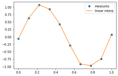
scipy.interpolate is useful for fitting a function from experimental data and thus evaluating points where no measure exists.

# Let's create some data
measured_time = np.linspace(0, 1, 10)
noise = (np.random.random(10)*2 - 1) * 1e-1
measures = np.sin(2 * np.pi * measured_time) + noise

scipy.interpolate.interp1d can build a linear interpolation function:

from scipy.interpolate import interp1d
linear_interp = interp1d(measured_time, measures)
interpolation_time = np.linspace(0, 1, 50)
linear_results = linear_interp(interpolation_time)

%matplotlib inline
from matplotlib import pyplot as plt
plt.plot(measured_time, measures, 'o', ms=6, label='measures')
plt.plot(interpolation_time, linear_results, label='linear interp')
plt.legend();

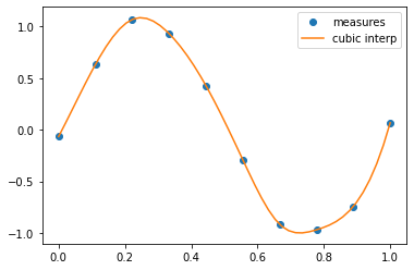
A cubic interpolation can also be selected by providing the kind optional keyword argument:

cubic_interp = interp1d(measured_time, measures, kind='cubic')
cubic_results = cubic_interp(interpolation_time)

plt.plot(measured_time, measures, 'o', ms=6, label='measures')
plt.plot(interpolation_time, cubic_results, label='cubic interp')
plt.legend()

<matplotlib.legend.Legend at 0x7f1e0bbe0fd0>

Optimization and fit: scipy.optimize

Optimization is the problem of finding a numerical solution to a minimization or equality.

The scipy.optimize module provides algorithms for function minimization (scalar or multi-dimensional), curve fitting and root finding.

from scipy import optimize

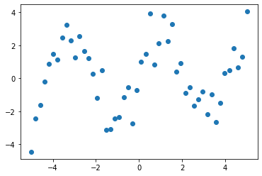
Curve fitting

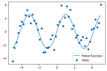
Suppose we have data on a sine wave, with some noise:

x_data = np.linspace(-5, 5, num=50)
y_data = 2.9 * np.sin(1.5 * x_data) + np.random.normal(size=50)

# And plot it
import matplotlib.pyplot as plt
plt.figure(figsize=(6, 4))
plt.scatter(x_data, y_data)
plt.show()

If we know that the data lies on a sine wave, but not the amplitudes or the period, we can find those by least squares curve fitting. First, we have to define the test function to fit, here a sine with unknown amplitude and period:

def test_func(x, a, b):
    return a * np.sin(b * x)

We then use scipy.optimize.curve_fit to find \(a\) and \(b\):

params, params_covariance = optimize.curve_fit(
    test_func, x_data, y_data, p0=[2, 2])
print(params)

[2.58100495 1.50430612]

# And plot the resulting curve on the data
plt.figure(figsize=(6, 4))
plt.scatter(x_data, y_data, label='Data')
plt.plot(x_data, test_func(x_data, params[0], params[1]),
         label='Fitted function')
plt.legend(loc='best')
plt.show()

Finding the minimum of a scalar function

Let’s define the following function:

def f(x):
    return x**2 + 10*np.sin(x)

and plot it:

x = np.arange(-10, 10, 0.1)
plt.plot(x, f(x))
plt.show()

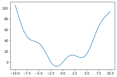
This function has a global minimum around -1.3 and a local minimum around 3.8.

Searching for minimum can be done with scipy.optimize.minimize, given a starting point x0, it returns the location of the minimum that it has found:

result = optimize.minimize(f, x0=0) 
result

      fun: -7.945823375615215
 hess_inv: array([[0.08589237]])
      jac: array([-1.1920929e-06])
  message: 'Optimization terminated successfully.'
     nfev: 18
      nit: 5
     njev: 6
   status: 0
  success: True
        x: array([-1.30644012])

result.x # The coordinate of the minimum

array([-1.30644012])

Fast Fourier transforms: scipy.fftpack

The scipy.fftpack module computes fast Fourier transforms (FFTs) and offers utilities to handle them. The main functions are:

• scipy.fftpack.fft to compute the FFT

• scipy.fftpack.fftfreq to generate the sampling frequencies

• scipy.fftpack.ifft computes the inverse FFT, from frequency space to signal space

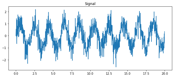
As an illustration, let’s create a (noisy) input signal (sig), and its FFT:

from scipy import fftpack

time_step = 0.02
period = 1. / 0.5  # 0.5 Hz

time_vec = np.arange(0, 20, time_step)
sig = (np.sin(2 * np.pi / period * time_vec)
       + 0.5 * np.random.randn(time_vec.size))

plt.figure(figsize=(10, 4))
plt.plot(time_vec, sig, label='Original signal')
plt.title('Signal')
plt.show()

# The FFT of the signal
sig_fft = fftpack.fft(sig)

# And the power (sig_fft is of complex dtype)
power = np.abs(sig_fft)

# The corresponding frequencies
sample_freq = fftpack.fftfreq(sig.size, d=time_step)

# Plot the FFT power
plt.figure(figsize=(10, 4))
plt.plot(sample_freq[:500], power[:500])
plt.xlabel('Frequency [Hz]')
plt.ylabel('plower')
plt.title('FFT')
plt.show()

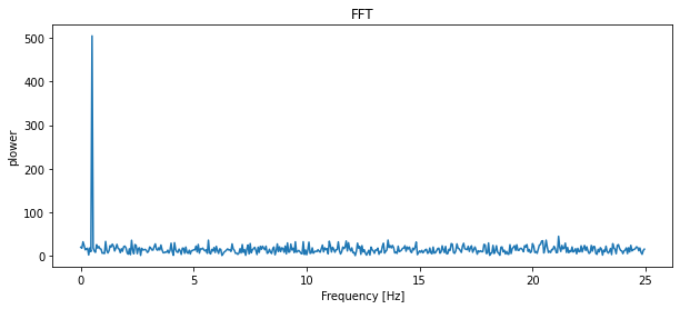
The peak signal frequency can be found with sample_freq[power.argmax()]

peak_freq = sample_freq[power.argmax()]
peak_freq

0.5

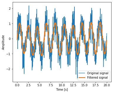
Setting the Fourier component above this frequency to zero and inverting the FFT with scipy.fftpack.ifft, gives a filtered signal:

high_freq_fft = sig_fft.copy()
high_freq_fft[np.abs(sample_freq) > peak_freq] = 0
filtered_sig = fftpack.ifft(high_freq_fft)

plt.figure(figsize=(6, 5))
plt.plot(time_vec, sig, label='Original signal')
plt.plot(time_vec, filtered_sig, linewidth=3, label='Filtered signal')
plt.xlabel('Time [s]')
plt.ylabel('Amplitude')
plt.legend(loc='best')
plt.show();

/opt/miniconda-latest/envs/neuro/lib/python3.7/site-packages/numpy/core/_asarray.py:85: ComplexWarning: Casting complex values to real discards the imaginary part
  return array(a, dtype, copy=False, order=order)

Signal processing: scipy.signal

scipy.signal is for typical signal processing: 1D, regularly-sampled signals.

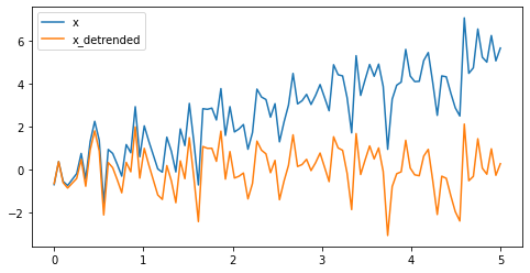
Detrending scipy.signal.detrend - remove linear trend from signal:

# Generate a random signal with a trend
import numpy as np
t = np.linspace(0, 5, 100)
x = t + np.random.normal(size=100)

# Detrend
from scipy import signal
x_detrended = signal.detrend(x)

# Plot
from matplotlib import pyplot as plt
plt.figure(figsize=(8, 4))
plt.plot(t, x, label="x")
plt.plot(t, x_detrended, label="x_detrended")
plt.legend(loc='best')
plt.show()

previous

Introduction to NumPy

next

Introduction to Visualization in python